Validation
So why should you trust in the high accuracy of the results presented here? To start with, the "functional" of the flow, the primary vortex intensity and its center coordinates, matches the generally accepted most accurate calculation available of Botella & Peyret (1998), [1] for Re = 1000, to all digits provided as seen on the previous page. It also matches Shapeev & Lin's (2008), [2] result extremely closely (less than 1.e-8 difference in the stream function value, with the center coordinates rather impressively agreeing to 8 digits).
A clarification of how the exact center is found is probably in order here. Most (all?) studies on the subject using finite difference methods, simply quote the value and coordinates of the grid point with the minimum stream function value. Obviously this will only be somewhere near the absolute minimum of the continuous solution. In contrast, the two referenced benchmark solutions are based on analytical approximating functions and thus it's possible to point to the predicted absolute minimum and its location. We can mimic that by focusing around the grid point with the minimum value, fit a few surrounding points with cubic interpolators and use a 2-D bisection kind of method to zone in on the "exact" location of the minimum (which will lie somewhere between the actual grid points). That said, I honestly did not expect to match somebody else's primary vortex coordinates to 8 digits. But cubic interpolation based on a very fine grid is apparently accurate enough for this (given of course the high quality and order of accuracy of both solutions).
Now this is already a good sign. But Botella & Peyret provide quite a bit more flow details, so let's make some more comparisons. Similarly to above, we need to interpolate in order to find the solution at the location points given in [1]. We use cubic splines for that. Incidentally, those are the locations originally used in the older paper by Ghia et. al. (1982), [3] whose results have served as the main reference for this test case ever since. Impressive for their time as those results were, given the much lower computational power of the 80s, nowadays there are unavoidably better resolved solutions out there. The present implementation only needs a few seconds of desktop time to produce much more accurate results.
So let's first look at how velocity and vorticity profiles match up through the centerlines of the cavity. The answer is pretty well. All velocity figures agree to the last digit and vorticity values are almost all identical as well.
Table 2. Velocity components and vorticity values through the centrelines of the cavity at Re = 1000, computed at the locations given in [1]
| x = 0.5 | y = 0.5 | |||||||||
| y | ux Ref. [1] | ux | ω Ref. [1] | ω | x | uy Ref. [1] | uy | ω Ref. [1] | ω | |
| 1 | 1 | 1 | -14.7534 | -14.7534 | 1 | 0 | 0 | 5.46217 | 5.46216 | |
| 0.9766 | 0.6644227 | 0.6644227 | -12.067 | -12.0670 | 0.9688 | -0.2279225 | -0.2279225 | 8.4435 | 8.44350 | |
| 0.9688 | 0.5808359 | 0.5808359 | -9.49496 | -9.49495 | 0.9609 | -0.2936869 | -0.2936869 | 8.24616 | 8.24616 | |
| 0.9609 | 0.5169277 | 0.5169277 | -6.95968 | -6.95966 | 0.9531 | -0.3553213 | -0.3553213 | 7.58524 | 7.58524 | |
| 0.9531 | 0.4723329 | 0.4723329 | -4.85754 | -4.85753 | 0.9453 | -0.4103754 | -0.4103754 | 6.50867 | 6.50867 | |
| 0.8516 | 0.3372212 | 0.3372212 | -1.762 | -1.76199 | 0.9063 | -0.5264392 | -0.5264392 | -0.92291 | -0.92291 | |
| 0.7344 | 0.1886747 | 0.1886747 | -2.09121 | -2.09121 | 0.8594 | -0.4264545 | -0.4264545 | -3.43016 | -3.43016 | |
| 0.6172 | 0.0570178 | 0.0570178 | -2.06539 | -2.06539 | 0.8047 | -0.3202137 | -0.3202137 | -2.21171 | -2.21171 | |
| 0.5 | -0.0620561 | -0.0620561 | -2.06722 | -2.06722 | 0.5 | 0.0257995 | 0.0257995 | -2.06722 | -2.06722 | |
| 0.4531 | -0.1081999 | -0.1081999 | -2.06215 | -2.06215 | 0.2344 | 0.3253592 | 0.3253592 | -2.06122 | -2.06122 | |
| 0.2813 | -0.2803696 | -0.2803696 | -2.26772 | -2.26772 | 0.2266 | 0.3339924 | 0.3339924 | -2.00174 | -2.00174 | |
| 0.1719 | -0.3885691 | -0.3885691 | -1.05467 | -1.05466 | 0.1563 | 0.3769189 | 0.3769189 | -0.74207 | -0.74207 | |
| 0.1016 | -0.3004561 | -0.3004561 | 1.63436 | 1.63436 | 0.0938 | 0.3330442 | 0.3330442 | 0.82398 | 0.82398 | |
| 0.0703 | -0.2228955 | -0.2228955 | 2.20175 | 2.20175 | 0.0781 | 0.3099097 | 0.3099097 | 1.23991 | 1.23991 | |
| 0.0625 | -0.20233 | -0.2023300 | 2.31786 | 2.31786 | 0.0703 | 0.2962703 | 0.2962703 | 1.50306 | 1.50306 | |
| 0.0547 | -0.1812881 | -0.1812881 | 2.4496 | 2.44960 | 0.0625 | 0.2807056 | 0.2807056 | 1.83308 | 1.83308 | |
| 0 | 0 | 0 | 4.16648 | 4.16648 | 0 | 0 | 0 | 7.66369 | 7.66368 | |
Next let's have a look at the extrema of the velocities through the centerlines of the cavity. Again here we fit cubic splines through the grid points in order to find the local extrema. Like before we have an almost perfect match, with just the last figure (vmin) differing by 1.5e-7.
Table 3. Extrema of the velocity components through the centerlines of the cavity at Re = 1000
| Work | umin | ymin | vmax | xmax | vmin | xmin |
| Present | -0.3885698 | 0.1716968 | 0.3769447 | 0.1578365 | -0.5270773 | 0.9092470 |
| Botella & Peyret [1] | -0.3885698 | 0.1717 | 0.3769447 | 0.1578 | -0.5270771 | 0.9092 |
Now let's move right to the boundaries. Something that might be more difficult to calculate with high accuracy is the vorticity on the moving lid (i.e. at Y = 1), especially near the two singularities (the corners where the moving lid meets the stationary side walls). That's in table 4 where again a near-perfect match is observed. We next focus even closer to the singularities in table 5 where we look at the vorticity on the side wall near the top right corner at two different points, first at (1, 0.95) and then for a proper torture test at (1, 0.999). Once again the results agree perfectly save for the most extreme point at (1, 0.999), but even there the difference is 0.04%. Let's remember that Botella & Peyret apply special treatment for the corners, the accuracy being achieved thanks to the subtraction of the leading part of the singularity. Here there is no special treatment (other than refining the grid near the boundaries), so a difference of only 0.04% that close to the singularity is remarkable. More so if we think that we are basically using vanilla flavor second order finite differences, though one has to be reminded that more than a day is needed to get this result even on a powerful modern PC.
|
Table 4. Vorticity values on the moving lid (Y=1) at Re = 1000, computed at the locations given in [1]
|
Table 5. Vorticity values on the side wall near the top right corner at
Re = 1000 |
|
|
Finally let's have a look at what lurks in the cavity's (stationary) corners. That's a series of counter-rotating vortices which decrease in size and intensity as the corner point is approached. As it is usually done in the literature, we will call the first (and largest) such vortex forming at the bottom right corner BR1. Botella & Peyret call it lower right secondary vortex. The second is called BR2 (or lower right tertiary vortex), the third one BR3, etc. Same for the left corner. So just how accurately are these smaller structures predicted by the present work? Table 6 has the lowdown. Apart from Botella & Peyret [1], I also reference the results of Shapeev & Lin [2] whose specialized treatment aims exactly at the (very) accurate prediction of these vortices (employing an exponentially refined grid in the corners and 6th order accuracy among other things). The primary vortex (PV) is also included for completeness. Once again the agreement with the two most accurate references is extremely close. It's only the third tier vortices BR3 and BL3 where the present results concede some accuracy to [2], but that's to be expected as these very fine structures appear at the grid frequency (smallest grid spacing for the present results is about 2.e-4). It is obviously hard to compute a vortex very accurately when it lies just one grid point from the corner. The relatively larger discrepancy (especially for the vorticity values) with Botella & Peyret is due to the fact that they actually calculate values at the rounded (to 4 digits) locations (x,y) they provide. This became obvious when the present solution was interpolated at those rounded locations (instead of the more accurate locations used and shown in table 6), which resulted in an almost perfect agreement (not shown here).
Table 6. Comparison of vortex intensities and locations at Re = 1000
| Present | Shapeev & Lin [2] | Botella & Peyret [1] | ||
| PV | ψ | -0.118936603 | -0.118936611 | -0.1189366 |
| ω | -2.067748 | - | -2.067750 | |
| x | 0.53079011 | 0.530790112 | 0.5308 | |
| y | 0.56524055 | 0.565240557 | 0.5652 | |
| BR1 | ψ | 0.001729717 | 0.001729717 | 0.00172971 |
| ω | 1.109259 | - | 1.109789 | |
| x | 0.86404005 | 0.86404006 | 0.864 | |
| y | 0.11180617 | 0.11180617 | 0.1118 | |
| BL1 | ψ | 0.0002334529 | 0.0002334529 | 0.000233453 |
| ω | 0.352093 | - | 0.352286 | |
| x | 0.08327318 | 0.08327318 | 0.0833 | |
| y | 0.078095722 | 0.078095725 | 0.0781 | |
| BR2 | ψ | -5.03935E-08 | -5.03938E-08 | -5.03944E-08 |
| ω | -0.0084223 | - | - | |
| x | 0.992324832 | 0.992324852 | 0.99232 | |
| y | 0.007650975 | 0.007650979 | 0.00765 | |
| BL2 | ψ | -6.39843E-09 | -6.39855E-09 | -6.39800E-09 |
| ω | -0.0026762 | - | - | |
| x | 0.004842621 | 0.004842696 | 0.00484 | |
| y | 0.004845120 | 0.004845241 | 0.00484 | |
| BR3 | ψ | 1.3073E-12 | 1.38949E-12 | - |
| ω | 6.5239E-05 | - | - | |
| x | 0.999534 | 0.9995375 | - | |
| y | 0.000466078 | 0.0004625364 | - | |
| BL3 | ψ | 1.55034E-13 | 1.76426E-13 | - |
| ω | 1.5756E-05 | - | - | |
| x | 0.000271489 | 0.0002923789 | - | |
| y | 0.000271488 | 0.0002923791 | - | |
The comparisons above broadly indicate that the Re 1000 solution is converged to 7 digits. Let us now have a look at higher Reynolds numbers. Compared to the Re 1000 case, solutions available to this problem for moderate to high Re tend to be far less grid-converged. In terms of the level of accuracy we are seeking here, there is only Shapeev & Lin (2008), [2] to compare with. So we will have to use vortex intensities and locations. As table 7 below demonstrates, the agreement is still extremely good, but does gradually become less close as Re goes up. Shapeev & Lin indicate that there is a (relative) deterioration in the accuracy of their solutions for high Reynolds numbers, attributed to the fact that their grid is only refined near the corners and thus cannot resolve the boundary layers as well as a grid which is refined all along the boundaries. They also imply that their high Re solutions are less grid-converged. In order to provide some indication of how well-converged the present benchmarks are, the results of the first (single) Richardson extrapolation (combining the 1201x1201 and 1413x1413 solutions), as well as those of the base second order 1201x1201 solution, are also shown. The latter is surprisingly well-preforming on its own, as was briefly suggested in the front page. In order to give some idea of its relative accuracy, 4th-order solutions courtesy of Erturk & Gokcol (2006), [5] are also included for comparison. It can be seen that the present 2nd-order 1201x1201 graded grid solutions are significantly more accurate than the 4th-order 601x601 uniform grid solutions, especially so as Re increases. This is rather unexpected and could be attributed partly to the presence of the singularities which "pollute" the solution and seem to prevent a scheme from performing according to its theoretical order. Refining the grid near the singularities goes a long way towards remedying this problem.
Table 7. Convergence and comparison of primary vortex intensities and locations for different Reynolds numbers.
N is the number of grid points per dimension, BR stands for boundary-refined, CR for corner-refined and U for uniform
N is the number of grid points per dimension, BR stands for boundary-refined, CR for corner-refined and U for uniform
| Re | Work | Method (order) | Grid(s) used | ψ | ω | x | y |
| 1000 | Present | FD (2) | N: 1201 BR | -0.1189363 | -2.067758 | 0.5307923 | 0.5652414 |
| Present | FD RE (2+) | N: 1201 & 1413 BR | -0.1189366 | -2.067748 | 0.5307901 | 0.5652405 | |
| Present | FD DRE (2+) | N: 1201 & 1413 & 1661 BR | -0.1189366 | -2.067748 | 0.5307901 | 0.5652406 | |
| Shapeev & Lin [2] | FE (6) | DOF: 226574 CR | -0.1189366 | - | 0.5307901 | 0.5652406 | |
| Erturk & Gokcol [4] | FD (4) | N: 601 U | -0.118938 | -2.067760 | 0.5300 | 0.5650 | |
| 2500 | Present | FD (2) | N: 1201 BR | -0.1214670 | -1.976054 | 0.5197794 | 0.5439247 |
| Present | FD RE (2+) | N: 1201 & 1413 BR | -0.1214689 | -1.976078 | 0.5197769 | 0.5439244 | |
| Present | FD DRE (2+) | N: 1201 & 1413 & 1661 BR | -0.1214689 | -1.976079 | 0.5197769 | 0.5439244 | |
| Shapeev & Lin [2] | FE (6) | DOF: 226574 CR | -0.1214690 | - | 0.5197769 | 0.5439244 | |
| Erturk & Gokcol [4] | FD (4) | N: 601 U | -0.121472 | -1.976132 | 0.5200 | 0.5433 | |
| 5000 | Present | FD (2) | N: 1201 BR | -0.1222215 | -1.940567 | 0.5150966 | 0.5352620 |
| Present | FD RE (2+) | N: 1201 & 1413 BR | -0.1222257 | -1.940634 | 0.5150939 | 0.5352619 | |
| Present | FD DRE (2+) | N: 1201 & 1413 & 1661 BR | -0.1222259 | -1.940636 | 0.5150938 | 0.5352620 | |
| Shapeev & Lin [2] | FE (6) | DOF: 226574 CR | -0.1222259 | - | 0.5150937 | 0.5352620 | |
| Erturk & Gokcol [4] | FD (4) | N: 601 U | -0.122216 | -1.940547 | 0.5150 | 0.5350 | |
| 7500 | Present | FD (2) | N: 1201 BR | -0.1223800 | -1.926834 | 0.5131001 | 0.5318915 |
| Present | FD RE (2+) | N: 1201 & 1413 BR | -0.1223864 | -1.926937 | 0.5130976 | 0.5318916 | |
| Present | FD DRE (2+) | N: 1201 & 1413 & 1661 BR | -0.1223865 | -1.926940 | 0.5130975 | 0.5318917 | |
| Shapeev & Lin [2] | FE (6) | DOF: 226574 CR | -0.1223867 | - | 0.5130967 | 0.5318922 | |
| Erturk & Gokcol [4] | FD (4) | N: 601 U | -0.122344 | -1.926478 | 0.5133 | 0.5317 | |
| 10000 | Present | FD (2) | N: 1201 BR | -0.1223910 | -1.919089 | 0.5119054 | 0.5300248 |
| Present | FD RE (2+) | N: 1201 & 1413 BR | -0.1223992 | -1.919221 | 0.5119033 | 0.5300250 | |
| Present | FD DRE (2+) | N: 1201 & 1413 & 1661 BR | -0.1223994 | -1.919226 | 0.5119032 | 0.5300251 | |
| Shapeev & Lin [2] | FE (6) | DOF: 226574 CR | -0.1223999 | - | 0.5119015 | 0.5300262 | |
| Erturk & Gokcol [4] | FD (4) | N: 601 U | -0.122306 | -1.918187 | 0.5117 | 0.5300 | |
| 12500 | Present | FD (2) | N: 1201 BR | -0.1223548 | -1.913955 | 0.5110750 | 0.5288036 |
| Present | FD RE (2+) | N: 1201 & 1413 BR | -0.1223645 | -1.914114 | 0.5110735 | 0.5288039 | |
| Present | FD DRE (2+) | N: 1201 & 1413 & 1661 BR | -0.1223648 | -1.914118 | 0.5110734 | 0.5288040 | |
| Shapeev & Lin [2] | FE (6) | DOF: 226574 CR | -0.1223661 | - | 0.5110722 | 0.5288052 | |
| Erturk & Gokcol [4] | FD (4) | N: 601 U | -0.122201 | -1.912307 | 0.5117 | 0.5283 | |
| 20000 | Present | FD (2) | N: 1201 BR | -0.1221800 | -1.905105 | 0.5095341 | 0.5267405 |
| Present | FD RE (2+) | N: 1201 & 1413 BR | -0.1221929 | -1.905314 | 0.5095350 | 0.5267408 | |
| Present | FD DRE (2+) | N: 1201 & 1413 & 1661 BR | -0.1221933 | -1.905322 | 0.5095348 | 0.5267410 | |
| Shapeev & Lin [2] | FE (6) | DOF: 226574 CR | -0.1222021 | - | 0.5095672 | 0.5267332 | |
| Erturk & Gokcol [4] | FD (4) | N: 601 U | -0.121694 | -1.900032 | 0.5100 | 0.5267 | |
| 25000 | Present | FD (2) | N: 1201 BR | -0.1220586 | -1.901634 | 0.5088824 | 0.5259503 |
| Present | FD RE (2+) | N: 1201 & 1413 BR | -0.1220726 | -1.901858 | 0.5088853 | 0.5259505 | |
| Present | FD DRE (2+) | N: 1201 & 1413 & 1661 BR | -0.1220731 | -1.901866 | 0.5088852 | 0.5259507 | |
| Shapeev & Lin [2] | FE (6) | DOF: 226574 CR | -0.1220905 | - | 0.5089511 | 0.5259381 | |
| Erturk & Gokcol [4] | FD (4) | N: 601 U | - | - | - | - | |
| 30000 | Present | FD (2) | N: 1201 BR | -0.1219451 | -1.899095 | 0.5083823 | 0.5253746 |
| Present | FD RE (2+) | N: 1201 & 1413 BR | -0.1219592 | -1.899317 | 0.5083874 | 0.5253747 | |
| Present | FD DRE (2+) | N: 1201 & 1413 & 1661 BR | -0.1219599 | -1.899328 | 0.5083872 | 0.5253750 | |
| Shapeev & Lin [2] | FE (6) | DOF: 226574 CR | - | - | - | - | |
| Erturk & Gokcol [4] | FD (4) | N: 601 U | - | - | - | - |
We can also perform a different kind of accuracy and health check by looking at the conservation of mass (continuity) of the flow. We can do that by calculating the net volumetric flow rate through any cross section of the cavity (or indeed any closed control volume inside the cavity). Since these are steady-state solutions and the flow is incompressible, any such flow rate should amount to zero. For example we can calculate the net flow rates through the vertical and horizontal centerlines of the cavity by integrating along them the horizontal and vertical velocity component respectively. We use cubic splines for the integration and we expect the result to be a really low number, given the accuracy of the present calculations and the density of the grid which should minimize any errors caused by the integration itself. As table 8 demonstrates, those are indeed really low values (highlighted in blue), providing further evidence of the high accuracy of the present solutions. The flow rates for the base second order solution and the first (single) Richardson Extrapolation are also shown. Since RE is applied to the computed node variables individually with no regard to the discretized equations they need to satisfy, one can be suspicious of the effect it might have on a global conservation quantity, like mass in this case. But as table 8 shows, RE is consistently and predictably working its magic here, drastically reducing the flow rate residual by way of significantly reducing the error on each individual grid point. Another interesting observation is that while the flow residuals through the vertical centerline (Qv) increase with Re, the opposite holds for the flow residuals through the horizontal centerline (Qh). A possible explanation is that while Qv is dominated by the very thin boundary layer on the lid, resulting in a slight error increase at higher Re, the boundary layers on the side walls just become thin enough at higher Re to move closer to the walls and be more accurately resolved by the higher available grid resolution there.
Table 8. Volumetric flow rates across the vertical and horizontal centerlines of the cavity for different Reynolds numbers, for the base second order, single RE and double RE (benchmark) solutions
| Re | |||||||||||
| Solution | 1000 | 2500 | 5000 | 7500 | 10000 | 12500 | 20000 | 25000 | 30000 | ||
| Qv | Base | 7.07E-07 | 6.91E-07 | 8.12E-07 | 9.36E-07 | 1.05E-06 | 1.16E-06 | 1.44E-06 | 1.60E-06 | 1.75E-06 | |
| RE | 1.07E-10 | 6.30E-10 | 8.27E-10 | 9.07E-10 | 9.58E-10 | 1.01E-09 | 1.18E-09 | 1.38E-09 | 1.67E-09 | ||
| DRE | 2.24E-11 | 1.24E-10 | 1.65E-10 | 1.83E-10 | 1.96E-10 | 2.07E-10 | 2.37E-10 | 2.59E-10 | 2.81E-10 | ||
| Qh | Base | -2.28E-07 | -1.76E-07 | -1.82E-07 | -2.04E-07 | -2.29E-07 | -2.55E-07 | -3.31E-07 | -3.77E-07 | -4.20E-07 | |
| RE | 6.45E-10 | 4.02E-10 | 2.97E-10 | 2.52E-10 | 2.27E-10 | 2.14E-10 | 2.15E-10 | 2.32E-10 | 2.51E-10 | ||
| DRE | 1.21E-10 | 7.48E-11 | 5.51E-11 | 4.64E-11 | 4.09E-11 | 3.67E-11 | 2.67E-11 | 2.06E-11 | 1.41E-11 | ||
Finally we can go back to the kind of torture test of table 5 and see how the high Re solutions may be affected by the singularities very near the top corners. There are no results in the literature to compare with as was the case for Re = 1000, but we can at least perform a visual check for numerical artifacts/oscillations. Figure 1 shows a magnification of the vorticity contours near the top two corners for the most "difficult" case considered here, i.e. for Re = 30000. As can be seen, there is no indication (at least visual) of the solution being affected by the singularities, even very near the corners. The solutions for all the other Reynolds numbers can be similarly inspected by zooming (up to 64 times) on the high resolution graphs included with the solutions pdfs in the Driven Cavity Benchmarks page.
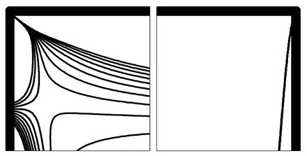
Figure 1. Vorticity contour magnifications near the top left and right corners (2% of each cavity side shown) for Re = 30000.
So we have established the benchmark-worthy accuracy of the results presented here, by way of (practically exactly for Re <= 10000) matching the two most accurate references available. Botella & Peyret (1998), [1] only solve for Re <= 1000 and Shapeev & Lin (2008), [2] only provide vortex information. In the present work the same level of accuracy is maintained, but detailed results such as various velocity and vorticity profiles, including near boundary layers, as well as vortex intensities are provided up to Re = 30000. Solution data at any other location are also available at request. The accuracy level should be consistent throughout the flow field, and at least for the higher Reynolds numbers improving on [2], as suggested above.
Now let's have a look at what happens when we use half as many grid points in each dimension, i.e. use a base grid of 601x601 and let's also make it uniform. This actually brings down the computational time to only a small fraction of what it takes to produce the benchmark results. Figure 2 shows how the solution typically converges as the grids' resolution is increased and we go from single to double Richardson extrapolation. So for the first curve the result is the composite of two runs on two uniform grids of sizes 601x601 and 510x510. The last curve (going back to higher resolution but included here to showcase the convergence trend) represents the composite of three runs on uniform grids of sizes 1201 x 1201, 1413 x 1413 and 1661 x 1661. As can be seen, the convergence is steady and monotonic. The error is calculated as the percentage difference from the results in [1], or indeed from the present benchmark solution which is identical as we saw in table 2. So if for the last case in figure 2 non-uniform grids are used instead, the error curve flattens to zero.
This graph also provides a way of estimating the remaining error in the benchmark (double RE) solutions through a comparison with the corresponding single RE results in table 7. We can see in figure 2 that the error of a double RE solution incorporating a third, finer grid (fourth curve) is about 3-4 times smaller than the difference between that solution and the single RE solution that only uses the first two grids (second curve). Although perhaps we cannot readily apply this result to the graded grid high Re simulations, a look at table 7 would suggest that the remaining error in the benchmark solutions should indeed be very small even for the high Re results.
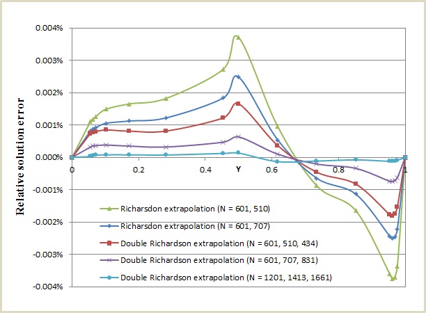
Figure 2. Solution convergence with varying uniform grid sizes and levels of Richardson extrapolation. for the horizontal velocity Ux through the vertical centreline (X=0.5) of the cavity, at Re = 1000.
As mentioned above, pretty heavy computations were required to produce the most accurate results presented here. That is the result of the high grid point count (2.75million for the largest grid used) and the very small spacing of the graded grids near the boun-daries, which necessitates the use of an accordingly low time-step in order to avoid divergence. Also since we are seeking many digits of accuracy, we have to use a very strict convergence criterion so that those digits do not change further. The quantity used to check convergence in the present work was the mean change in vorticity values between successive time-steps and for the benchmark runs I let this "residual" fall to 1.e-13.
On the other hand, a simulation on a 300x300 grid takes less than a minute to converge and yields more than enough accuracy for practical purposes. The effect that the use of Richardson Extrapolation (RE) and non-uniform grids have on the accuracy of the solution is illustrated in figure 3. The error like before is the percentage difference from the benchmark solution and the timings are on a 2009 desktop PC.
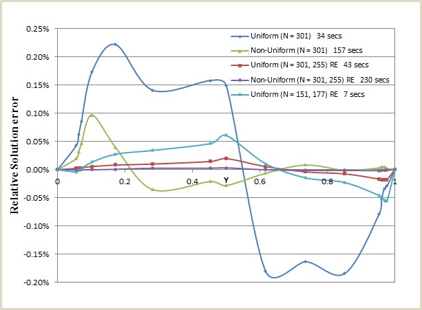
Figure 3. Solution error and timings for moderate size uniform and non-uniform grids, with and without Richardson Extrapolation, for the horizontal velocity Ux through the vertical centreline (X=0.5) of the cavity, at Re = 1000.
It can be seen that RE greatly improves the base solution accuracy on both uniform and non-uniform grids. Using a non-uniform grid on its own significantly reduces the overall error compared to the same size uniform grid run, especially near the lid where it matters, though it takes a lot more time. That said, it can be seen that there are areas where the grid's non-uniformity combines with high local derivatives of the solution to produce local error spikes (2nd curve at Y = 0.1). This is an inevitable problem, but can be mitigated by choosing a grid with reasonably smooth gradation. For the present work I have chosen moderately graded grids, in an effort to keep the benefits of the better resolved boundaries without introducing large local errors or compromising the accuracy at the centre. It can be seen that RE does work equally well with the symmetrically non-uniform grid in this simple geometry, with a single application totally eliminating the local error spike as the 4th curve shows. The convergence criterion for these non-benchmark calculations was 1.e-9, which was low enough relative to the discretization errors, with the exception of the results corresponding to the 4th curve where 1.e-10 was needed in order to match the much lower discretization error. Finally for a cost-effective solution, the uniform 151 x 151 grid run with RE cannot be beaten, producing a solution with maximum relative error of about 0.05% in a few seconds. To put this into perspective, the maximum error of the older benchmark results of Ghia et. al. was 2%.
Page 3: Discussion