A Driven Cavity Exploration by Yiannis Papadopoulos, June 2015
CFD (Computational Fluid Dynamics) was my favorite subject during my Mechanical Engineering studies. I was immediately impressed by the fact that one can use those simple laws we were taught in school physics to actually "simulate" real, complicated phenomena. All that one needed was a computer and basic programming skills. And there were loads of numbers to look at in the end. I like numbers. I ended up doing my final thesis simulating shock wave - boundary layer interactions, all by basically applying the conservation of mass, momentum and thermal energy principals to a bunch of little ("finite") volumes. That was quite an advanced affair, certainly for an undergraduate, and I thoroughly enjoyed it. But there was this much simpler (and almost equally interesting) test case that I had come across, that I didn't get to solve at the time: the famous (for CFD people anyway) "lid-driven square cavity" flow. Basically one has a square duct covered by a lid that slides sideways, sweeping the fluid (say air, or water) inside the duct and thus setting it in cross-sectional motion. This is a very easy problem to program and solve, yet what is revealed to be happening inside the cavity is surprising and looks rather impressive. So when a few years later I took time off from my non-related job (in finance), I sat down to solve this like I always wanted to, just for fun. I also wrote a small application to graphically represent the results and help me run the experiments. I then forgot the whole thing in the hard disk for more than a decade, until recently when I found myself with free time again and revisited it. I quickly realized that I still find all this quite entertaining so I guess I got carried away, spending most of the winter in front of the computer refining my previous effort, determined to get to the bottom, or should I say the corners of this (and gaining a few kilos in the process!).
The result was a new set of driven cavity flow benchmark solutions that should stand out from the existing literature as being the only practically grid-converged even for high Reynolds numbers, making them the most accurate available. Here I am sharing those solutions and I may share the app as well at some point in the future since visualizing the solution progress in time provides some useful insight.
My motivation is double: First, having spent quite a bit of time working on this, I thought it would be wasteful if nobody ever saw the results. So I hope that a few people find something interesting and useful here. Second, even though there are hundreds of papers on this subject, there seems to be a lack of really accurate, benchmark solutions. There is one paper by Botella & Peyret, (1998) [1] who do present highly accurate results for Reynolds number up to Re = 1000, for a few selected points/sections of the flow field. But for Re > 1000 there don't seem to be "definitive" results out there and divergence between different sources grows with the Reynolds number. Researchers often note this lack of benchmark results for Re>1000 and use their own solutions obtained on a fine grid as reference. Here I am trying to fill this gap by offering the same very high level of accuracy as in [1], all the way up to up to Re = 30000. And if the usual tabulated results at various points/sections of the flow don't cover your benchmarking needs, any other solution data can be provided upon request.
For the Re = 1000 case, Botella's and Peyret's results are indeed reproduced by the present work to the last digit. Given that the method (spectral) used in their work is completely different to the method used here, the exact match suggests both solutions are equally highly accurate. For the high Re solutions presented here the accuracy (i.e. grid-convergence) is probably down marginally, but should still be above anything else currently published by at least 1-2 orders of magnitude.
Numerical solution
The method used here is one of the oldest applied to this problem, so nothing innovative to report on this front. We are solving the time-dependent Navier-Stokes equations in their vorticity - stream function formulation, using second order (all central) finite difference discretizations, coupled with second order boundary conditions (as per Jensen). So full second order spatial accuracy can be expected. The solution is advanced in time through the vorticity transport equation with the ADI method starting from zero (simulating an impulsively started lid) until a steady state is reached. The stream function equation is not solved to high accuracy at each time-step so the validity of the intermediate solution stages is questionable, although they do look "realistic" when they are visualized. As stated above, the purpose here is to find the final steady state with high accuracy.
But I hear you already, how can you match Botella & Peyret's spectral results to 7 digits using a second order scheme with anything less than a prohibitively huge grid? And likewise, how come you compute more accurate solutions than others existing for high Re with such a mundane scheme? This is where another mundane trick comes to help, Richardson Extrapolation (RE). The use of RE for improving a solution's accuracy is often cautioned against but don't let this put you off, as we will see it really works well in this (simple) case. RE is used to calculate a highly accurate solution on all of the original grid points. To produce the benchmark solutions presented here, three different large (graded) grids were used (of sizes 1201x1201, 1413x1413 and 1661x1661) and the extrapolated result was projected (interpolated) onto the base 1201x1201 grid. The total calculation time for each Reynolds case was a few days on a 2009 i7-920 PC running at 100%.
Contributing to the final accuracy is, as just mentioned, the use of graded grids. Using higher resolution near the boundaries has a significant effect on the accuracy, not only locally near the boundaries (as expected), but also rather surprisingly in the main flow area. This is because vorticity is generated at the upper boundary (by the moving lid) and from there transported and diffused to the rest of the cavity. Thus more accurate modelling of this process presumably leads to better vorticity prediction everywhere in the flow field. High grid resolution near the corners also ensures that any small corner eddies that may affect the main flow are properly resolved.
Finally, it is worth noting that not all nominally second-order implementations are equally accurate, for various reasons. For example, a conservative scheme is usually more accurate than a non-conservative variant of the same order. Here the building block for the final composite solution, i.e. the base second-order solution, is on its own right surprisingly highly accurate as we shall see on the next page.
Results
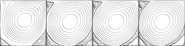
The main flow characteristic of this problem (at least for the Reynolds numbers considered here) is a large vortex which forms at the centre of the cavity and dominates the flow field. This is called the primary vortex since there are a lot more smaller ones squeezed in the corners. It thus makes sense to choose the intensity (and location) of the primary vortex centre, as the "functional" to use in order to summarize the calculation and determine the overall accuracy and grid convergence of the result.
So without further ado, here is a summary of the calculations. Full solution details on the Driven Cavity Benchmarks page.
So without further ado, here is a summary of the calculations. Full solution details on the Driven Cavity Benchmarks page.
Table 1. Overview of results: Calculated intensity and location of the primary vortex compared to other highly accurate references
| Re | ψ | ω | x | y |
| 1000 | -0.118936603 | -2.0677479 | 0.53079011 | 0.56524055 |
| Shapeev & Lin (2008), [2] | -0.118936611 | - | 0.530790112 | 0.565240557 |
| Botella & Peyret (1998), [1] N = 128 | -0.1189366 | -2.06775 | 0.5308 | 0.5652 |
| 2500 | -0.1214689 | -1.976079 | 0.5197769 | 0.5439244 |
| Shapeev & Lin (2008), [2] | -0.1214690 | - | 0.5197769 | 0.5439244 |
| 5000 | -0.1222259 | -1.940636 | 0.5150938 | 0.5352620 |
| Shapeev & Lin (2008), [2] | -0.1222259 | - | 0.5150937 | 0.5352620 |
| 7500 | -0.1223865 | -1.926940 | 0.5130975 | 0.5318917 |
| Shapeev & Lin (2008), [2] | -0.1223867 | - | 0.5130967 | 0.5318922 |
| 10000 | -0.1223994 | -1.919226 | 0.5119032 | 0.5300251 |
| Shapeev & Lin (2008), [2] | -0.1223999 | - | 0.5119015 | 0.5300262 |
| 12500 | -0.1223648 | -1.914118 | 0.5110734 | 0.5288040 |
| Shapeev & Lin (2008), [2] | -0.1223661 | - | 0.5110722 | 0.5288052 |
| 20000 | -0.1221933 | -1.905322 | 0.5095348 | 0.5267410 |
| Shapeev & Lin (2008), [2] | -0.1222021 | - | 0.5095672 | 0.5267332 |
| 25000 | -0.1220731 | -1.901866 | 0.5088852 | 0.5259507 |
| Shapeev & Lin (2008), [2] | -0.1220905 | - | 0.5089511 | 0.5259381 |
| 30000 | -0.1219599 | -1.899328 | 0.5083872 | 0.5253750 |
The second and third columns show the stream function and vorticity values respectively at the coordinates (x,y) of the center of the primary vortex (last two columns). Apart from Botella & Peyret's work, there is an interesting paper by Shapeev & Lin (2008), [2] who also seem to present very accurate results, up to Re = 25000, although they don't provide any velocity or vorticity profiles. Instead, they focus on the accurate prediction of intensities (stream function values) and location for the numerous (theoretically infinite) corner eddies/ vortices. So I am referencing those as well. In fact this has been a talking point of many papers on the subject, i.e. how many corner eddies one's calculation reveals. It's one way of assessing the quality of a simulation, looking at how accurately it predicts the smaller vortical structures. Obviously, the finer the grid the better it will resolve the finer structures for any given numerical scheme.
The singularities of the flow in the cavity corners (primarily the top corners where the velocity discontinuously changes from constant on the lid to zero on the walls) is another issue which affects both the accuracy and convergence behavior (and order) of the solution. The two studies referenced above do apply special treatment for this, while in the present work I do not. That said, the very fine grid used in the corners goes a long way towards minimizing any loss of accuracy there as we will see next.
Finally we should also briefly talk about the nature of the flow. Here, 2D steady-state solutions are presented, i.e. solutions to the Navier-Stokes equations with the time derivative set to zero. In general, being able to calculate a steady-state solution to a problem does not necessarily mean that this solution is stable (to finite perturbations), or indeed that it can be realized in a physical experiment. With computational power ever increasing, people have been able to compute steady-state solutions to this problem for higher Re numbers than before (up to Re = 65000 to my knowledge, in [10]). At the same time there are numerous studies suggesting this flow loses its stability at around Re = 8000. And the plot thickens further, because as it turns out the real physical flow would not be two-dimensional even at lower Re. So really most of the literature on this benchmark problem deals with a fictitious flow, useful for evaluating new Navier-Stokes solvers nonetheless. Some more discussion on this later.
This test case has been extensively studied and documented for decades and is probably not the current research flavor of the month. It does though still widely feature in new publications, mainly used for validating new numerical methods as mentioned above. So for whatever it is worth, here I present definitive 2-D steady solutions up to Re = 30000 to be used as reference whenever some new way of solving the N-S equations is being tested. If your solver can find a steady-state solution, then you can use the results presented here to assess the accuracy of your calculations, especially if you are testing for moderate to high Reynolds numbers and/or want to look closer to the boundary layers.
Go to the next page to see why there is good reason indeed you should trust these results.
Page 2: Validation