As promised in the previous post, I am going to present here some first results on using Deep Neural Networks (DNN's) for producing ultra fast (and accurate) approximations of complex structured product pricing models. That means: take the model currently used (whatever it may be) that is computationally expensive (Monte Carlo) and replace it with a lightning fast equivalent with the same (or maybe higher?) accuracy as that used in the production environment. As anticipated, this proved a more challenging and time-consuming undertaking than the stochastic volatility model calibration of the previous post. The end result though is still very satisfactory and has room for improvement given more resources. A surprise to me given the much higher dimensionality and discontinuous (in time) nature of the approximated (model pricing) function.
Since I do not currently have access to a proper production model (that could for example employ some Local Stochastic Volatility model for the underlying processes), I will use simple GBM. The number of free input parameters (dimensionality of the approximated function) is 28 (see below), which combined with the pricing discontinuities at the autocall dates still make for a very challenging problem. My experience so far (on training DNN's for simpler exotics) is that replacing GBM with a volatility model does not pose unsurmountable difficulties for the DNN. I am confident that similar (or higher) accuracy to the one showcased here can be achieved for the same MRBCA, at the expense of more (offline) effort in generating data and training the DNN.
Since I do not currently have access to a proper production model (that could for example employ some Local Stochastic Volatility model for the underlying processes), I will use simple GBM. The number of free input parameters (dimensionality of the approximated function) is 28 (see below), which combined with the pricing discontinuities at the autocall dates still make for a very challenging problem. My experience so far (on training DNN's for simpler exotics) is that replacing GBM with a volatility model does not pose unsurmountable difficulties for the DNN. I am confident that similar (or higher) accuracy to the one showcased here can be achieved for the same MRBCA, at the expense of more (offline) effort in generating data and training the DNN.
The product class
The product class we are looking at (autocallable multi barrier reverse convertibles) is popular in the Swiss market. It is a structured product paying a guaranteed coupon throughout its lifetime with a complex barrier option embedded. The latter is contingent on the worst performing out of a basket of underlying assets. There is a down-and-in type continuously monitored barrier and an up-and-out discretely monitored one (at the autocall dates). The assets' performance (level) is measured as a percentage of their initial fixing values. Accordngly, the strike level K for the down-and-in payoff, the down-and-in barrier B and the early redemption (autocall) level A (the "up-and-out barrier") are quoted as percentages.
In short: The product pays the holder a guaranteed coupon throughout its lifetime (up to maturity or early redemption). If on any of the observation (autocall) dates the worst-performing asset level is above the early redemption level, the product expires immediately and the amount redeemed is 100% of the nominal value. If no early redemption event happens then at maturity :
In short: The product pays the holder a guaranteed coupon throughout its lifetime (up to maturity or early redemption). If on any of the observation (autocall) dates the worst-performing asset level is above the early redemption level, the product expires immediately and the amount redeemed is 100% of the nominal value. If no early redemption event happens then at maturity :
- If during the lifetime of the product the worst-performing asset level did not at any moment touch or cross the barrier level B, the amount redeemed is 100% of the nominal value.
- If the worst-performing asset level did touch or cross the barrier level B at some point and its final fixing level is above the strike level K, the amount redeemed is again 100% of the nominal value.
- If the worst-performing asset did touch or cross the barrier level B at some point and its final fixing level is below the strike level K, the amount redeemed is the percentage of the nominal equal to the worst-performing asset performance (ratio of its final to initial fixing level).
The specific product to be approximated
I am not going to attempt an all-encompassing DNN representation of any possible MRBCA structure, but rather focus the effort on particular subcategory. So what I am looking for is a pricing approximation for MRBCA's on the worst of 4 assets, with original maturity of 2Y and semi-annual coupon payment and autocall dates. Also assuming the product is struck at-the-money (i.e. the strike level K is 100%, the most usual case in practice) with an early redemption (autocall) level of also 100%, again typical in the market. The latter two could of course also be included as variable inputs in the approximation. This may well be possible while maintaining the same accuracy but I haven't tried it yet.
So the DNN approximation will be for the clean price of any such product (given the inputs described next) at any time after its inception, up to its maturity. Indeed in what follows, T denotes the time left to maturity.
So the DNN approximation will be for the clean price of any such product (given the inputs described next) at any time after its inception, up to its maturity. Indeed in what follows, T denotes the time left to maturity.
28 model inputs - features for the DNN training
- The asset level S (% of initial fixing), volatility vol and dividend yield d for each of the 4 underlying GBM processes.
- Seven-point discount factor curve (1D, 1W, 1M, 3M, 6M, 1Y, 2Y).
- Time left to maturity T (in years).
- Barrier level B (% of initial fixings).
- Coupon level Cpn (% p.a.).
- Correlation matrix (six distinct entries).
The DNN is trained for wide ranges of its inputs to allow it to be used for a long time without the need for retraining. The approximation is only guaranteed to be good within the input ranges that it has been trained for. Those are shown below.
| Operational parameter ranges | ||||
| Min | Max | |||
| Si | 20% | 500% | ||
| voli | 10% | 40% | ||
| di | 0 | 10% | ||
| T | 0.001 | 2 | ||
| r (disc. rates) | -2% | 2.50% | ||
| B | 40% | 80% | ||
| Cpn | 2% p.a. | 20% p.a. | ||
| ρ | -55% | 99% | ||
Pricing model implementation
The original pricing model / function we aim to "mimic" is of course based on Monte Carlo simulation and was written in C++. I omitted things like date conventions and calendars for ease of implementation. The continuously monitored (American) down-and-in barrier feature is taken care of via the use of a probabilistic correction (Brownian Bridge). Given the assumed GBM processes, this not only perfectly eliminates any simulation bias, but also enables the use of large time-steps thus allowing for significant speedup in the generation of the training samples. The discount curve interpolation is based on cubic splines and auxiliary points. The simulation can be driven by either pseudo random numbers or quasi random sequences (Sobol). I chose the former for the generation of the training samples as it proved to be more beneficial for the learning ability of the DNN under my current setup.
Note that in contrast with the use case in the previous post, here the training output data (the MC prices) are noisy and of limited accuracy. Does this represent a big problem for the DNN's ability to learn from them? It turns out that the answer is not really.
Note that in contrast with the use case in the previous post, here the training output data (the MC prices) are noisy and of limited accuracy. Does this represent a big problem for the DNN's ability to learn from them? It turns out that the answer is not really.
DNN Training and validation
The DNN is trained by feeding it millions of [vector(inputs), price] pairs. This process in practice has to be repeated many times since there is no general formula for what works best in each case. The pricing accuracy of the training set samples does not have to be as high as the target accuracy. As it turns out the DNN has the ability to effectively smooth out the pricing data noise and come up with an accuracy that is higher than that on the individual prices it was trained on. Also the input space coverage does not have to be uniform as we may want for example to place more points where the solution changes rapidly in an effort to end up with a balanced error distribution.
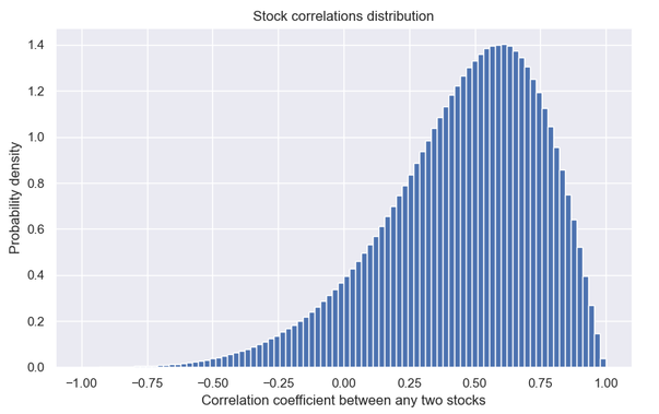
When it comes to testing the resulting DNN approximation though we create a separate (out of sample) test set of highly accurate prices uniformly filling the input space. This is to say we don't weigh some areas of the solution (say near the barrier) more than others when we calculate the error metrics. We say this is the operational (inputs) range of the DNN and we provide (or at least aim to) similar accuracy everywhere within that range. So the test set is created by drawing random inputs from uniform distributions within their respective ranges. The one exception being the correlation matrices whose coefficients follow the distribution below. We then discard those matrices that include coefficients outside our target range of (-55% to 99%).
When it comes to testing the resulting DNN approximation though we create a separate (out of sample) test set of highly accurate prices uniformly filling the input space. This is to say we don't weigh some areas of the solution (say near the barrier) more than others when we calculate the error metrics. We say this is the operational (inputs) range of the DNN and we provide (or at least aim to) similar accuracy everywhere within that range. So the test set is created by drawing random inputs from uniform distributions within their respective ranges. The one exception being the correlation matrices whose coefficients follow the distribution below. We then discard those matrices that include coefficients outside our target range of (-55% to 99%).
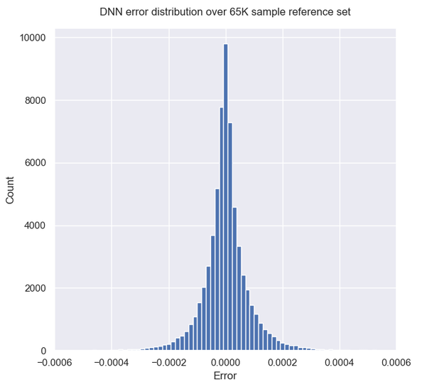
The overall accuracy achieved by the DNN is measured by the usual Mean Absolute Error (MAE) and Root Mean Square Error (RMSE) metrics. We can also look at the error distribution to get an idea of how good the approximation is. What we cannot easily do is say what lies far in the tails of that distribution, or in other words provide some sort of limit for the maximum possible error. In contrast to the traditional MC model, there is no theoretical confidence interval for the DNN error.
The MAE and RMSE are calculated against a reference test set of 65K MC prices, each generated using 32 million Sobol-driven paths (with Brownian Bridge construction). Such prices are found (when re-calculating a subset using 268 million Sobol paths) to have an accuracy of 4.e-6, which is well below the target accuracy (about 1.e-4, or 1 cent in a nominal of 100$). The inputs were generated again using (22-dimensional, correlations excluded) Sobol points, in an effort to best represent the space. The average model price for this test set is 0.874 (87.4%).
In order to try and get an idea for the worst-case errors I tested the DNN against a much bigger (but less accurate) test set of 16.7 million Sobol points.
DNN approximation performance
For the results presented here the DNN was trained on 80 million [vector(inputs), price] samples carefully chosen so as to ensure that error levels are as uniform as possible across the input space. At this training set size the convergence rate (error decrease with each doubling of training set size) was showing some signs of slowing down, but there was still room for improvement. Using a few hundred million samples would still be straightforward and would yield even better accuracy.
Still the overall quality of the approximation is excellent. The mean error is less than a cent and generally does not exceed 3 cents. The speed is as expected many orders of magnitude higher than an MC simulation with similar standard error (see below). The timings are for a single CPU core. Of course if GPU's are used instead the speed can still be improved significantly.
Still the overall quality of the approximation is excellent. The mean error is less than a cent and generally does not exceed 3 cents. The speed is as expected many orders of magnitude higher than an MC simulation with similar standard error (see below). The timings are for a single CPU core. Of course if GPU's are used instead the speed can still be improved significantly.
| Deep Neural Network Pricing Performance | ||||
| MAE | 6×10⁻⁵ | |||
| RMSE | 9×10⁻⁵ | |||
| Maximum absolute error in 16.7M test samples | 1.5×10⁻² | |||
| CPU time per price (1 core) | 6×10⁻⁶ secs | |||
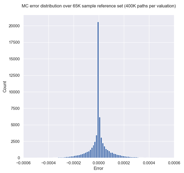
in order to get similar accuracy from the traditional MC model one needs about 400K antithetic paths. With the present implementation this takes about 0.35 secs on 1 CPU core, which is about 60000 times slower than the DNN. If the MC pricing employed some volatility model needing fine time steps, the speedup factor could easily be in the order of millions (the DNN speed would remain the same).
The MC model prices a lot of the samples with almost zero error. This is because for many of the random input parameter vectors the solution is basically deterministic and the product behaves either like a bond or is certain to be redeemed early.
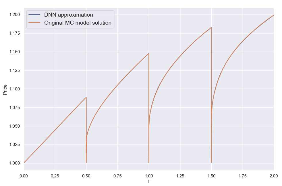
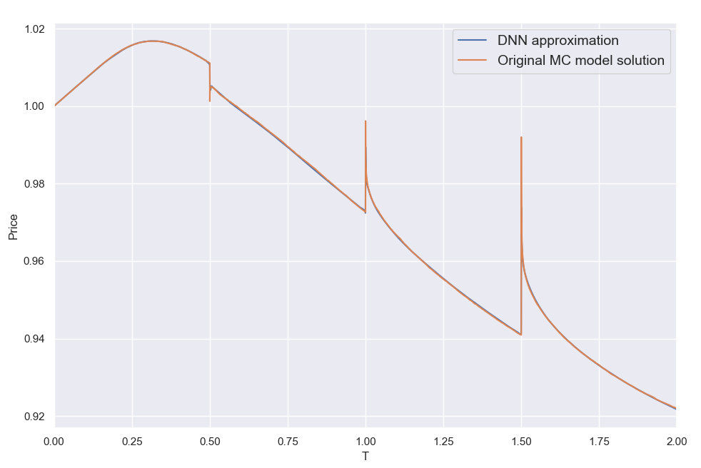
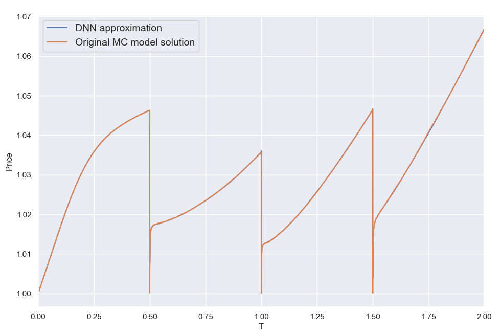
By far the most challenging dimension in the 28-dimentional function we are approximating here is the time to expiry T. The (clean) product price can be discontinuous at the autocall dates, posing a torture test for any numerical method. This is illustrated below where I am plotting a few sample solutions across T (keeping all other input parameters constant). These "pathological" cases correspond to the random input parameter vectors that resulted in the worst DNN approximation errors among the 16.7 million reference set cases (top 5 worst errors). The MC price plots are based on 40000 valuation points using 132K Sobol-driven paths per valuation. It took about 10 mins to create each plot utilizing all 12 cores of a CPU . The corresponding 40000 DNN approximations took < 0.2sec on a single core.
By far the most challenging dimension in the 28-dimentional function we are approximating here is the time to expiry T. The (clean) product price can be discontinuous at the autocall dates, posing a torture test for any numerical method. This is illustrated below where I am plotting a few sample solutions across T (keeping all other input parameters constant). These "pathological" cases correspond to the random input parameter vectors that resulted in the worst DNN approximation errors among the 16.7 million reference set cases (top 5 worst errors). The MC price plots are based on 40000 valuation points using 132K Sobol-driven paths per valuation. It took about 10 mins to create each plot utilizing all 12 cores of a CPU . The corresponding 40000 DNN approximations took < 0.2sec on a single core.
Looking at these plots it comes as no great surprise that the DNN struggles here. Considering the vast variety of shapes the solution can take, it is nonetheless seriously impressive that the DNN can cope as well as it does overall. That said, the maximum errors above are about 1.5% (not quite visible, located within those ultra narrow dips a few hours from the auto-call dates), which is more than I would have been happy with. Still, for use in XVA type calculations and intraday portfolio valuation monitoring, the performance is more than adequate as is. For use in a production environment one would need to be even more stringent with ensuring the maximum errors do not exceed a certain threshold. When testing the DNN against the much smaller 65K reference set, the maximum error was an order of magnitude smaller (about 0.2%, or 20 cents). Looking at 100M cases may reveal an even worse case than the 1.5% error found in the 16.7M set. Nonetheless there are ways to identify and target the problematic areas of the input parameter space. I am thus confident the maximum errors can be brought down further together with the mean error metrics by increasing and further refining the synthetic training set.
In conclusion, we can say that the DNN has passed this second much more difficult test as well. There was never a doubt that the approximation accuracy increases with increasing training data. The question in my mind was rather "is the sufficient amount of training (for the DNN to produce a worthy replacement of the traditional MC and PDE-based pricing) practical in terms of time and cost"? Given the experience gathered so far I would say the answer is yes. The present results were achieved mainly on a top spec desktop with only limited use of cloud resources. Approximating fully fledged models incorporating local and/or stochastic volatility will require more computational power, but the offline effort would still correspond to reasonable time and cost. To this end, a third post in this series would look at the case of FX TARF pricing under an LV or LSV model.
P.S. The results summarily presented in these last two posts are the culmination of a lot of work and experimentation that took the better part of a year and thousands of CPU/GPU hours.
 RSS Feed