In my previous post I talked about fast and accurate pricing of FX Target Redemption Forwards (TARF's) using the PDE/FDM method. I did that in a flat volatility (Black Scholes) setting to briefly show that even in this simple case there can be a big difference in the performance of the TARF pricing engine, depending on how considerate one is, God (or the devil) is in the details.
Let me clarify that here I am obviously talking about accuracy in terms of the discretization error of the numerical solution, not the model error. Just like a Monte Carlo simulation needs as many optimizations (and iterations) as one can afford in order to get an acceptably converged result, the same holds for finite difference/element methods (FDM/FEM) - just replace iterations with grid/mesh size.
Setting up the PDE-based TARF pricing engine properly is not trivial in its implemention and testing its convergencge properties with flat volatility should be the first step. But of course in most applications a volatility model is necessary. So in this post I will just take the engine I built for the previous post and instead of flat volatility use a (space and time-dependent) local volatility function a la Dupire. This is a pretty easy upgrade. After all the engine's building blocks are a bunch of individual 1-D BS PDE solvers and all we need to do is allow the volatility to be a function, nothing else has to change. The only question is how much would this affect the computational efficiency of the engine. As it turns out, not much at all, provided your local volatility surface is not discontinuous and too wild (and you cache and re-use some coefficients between the solvers).
Since I do not currently have access to market data, my brief tests here will be based on a sample market implied volatility (IV) surface sourced from [1] :
| Market data for USD/JPY from 11 June 2014 (spot = 102.00). Strikes implied assuming delta-neutral ATM type | |||||||||||||
| 10 Put | 25 Put | ATM | 25 Call | 10 Call | rates | ||||||||
| Mat | vol | strike | vol | strike | vol | strike | vol | strike | vol | strike | dom | for | |
| 1M | 6.08% | 99.7800 | 5.76% | 100.8834 | 5.53% | 101.9929 | 5.63% | 103.0908 | 5.81% | 104.1573 | -0.04% | 0.20% | |
| 3M | 7.08% | 97.4668 | 6.53% | 99.7695 | 6.15% | 101.9921 | 6.20% | 104.1550 | 6.44% | 106.3104 | 0.07% | 0.29% | |
| 6M | 8.19% | 94.7459 | 7.42% | 98.4743 | 6.95% | 102.0008 | 7.00% | 105.4620 | 7.36% | 109.0553 | 0.16% | 0.40% | |
| 1Y | 9.90% | 90.0345 | 8.61% | 96.3376 | 7.95% | 102.0061 | 8.04% | 107.6629 | 8.69% | 114.0638 | 0.21% | 0.52% | |
Local volatility surface construction
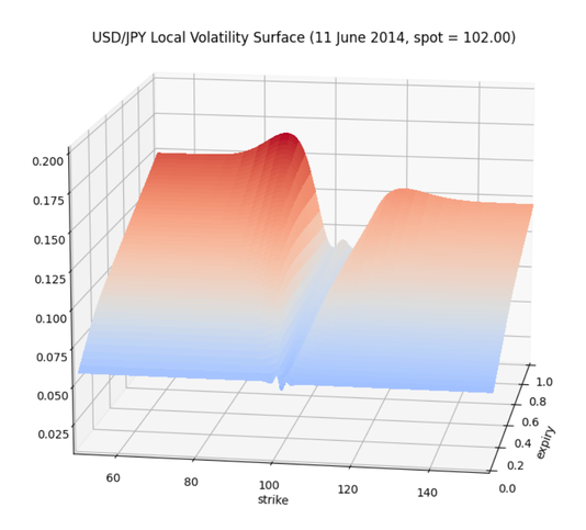
Without going into too much detail, the local volatility (LV) surface construction here is based on direct application of Dupire’s formula (using IV’s, not option values). To calculate the derivatives involved I calculated a fine grid of IV’s via interpolation of the market IV surface. For that I used Gaussian kernel interpolation in the delta dimension (later turned to strike scale). Such an approach by construction guarantees no arbitrage on single smiles and has an inherent extrapolation method (as suggested in [2]). In the time dimension I used cubic spline interpolation. For my sample IV surface this is just fine, but generally it could lead to calendar arbitrage and thus something more sophisticated would be used in practice to make sure of that. Either way, the LV surface construction is not the focus of this post, so I am assuming there is a good one available. Obviously the smoother the resulting surface, the smaller the negative effect on the finite difference scheme discretization error.
For the purpose of the present test I used 300 x 400 points in the strike and time dimension respectively (shown below). Most of the points in the strike dimension are placed around the spot. The above LV calibration procedure takes about 20 milliseconds. This surface is then interpolated (bi-)linearly by each solver to find the required local volatility function values on the pricing grid points. As for the quality of the calibration, using the same LV-enabled 1-D FD solvers making up the TARF pricing engine to price the market vanillas, produces an almost perfect fit in this case (IV RMSE about 0.001%).
For the purpose of the present test I used 300 x 400 points in the strike and time dimension respectively (shown below). Most of the points in the strike dimension are placed around the spot. The above LV calibration procedure takes about 20 milliseconds. This surface is then interpolated (bi-)linearly by each solver to find the required local volatility function values on the pricing grid points. As for the quality of the calibration, using the same LV-enabled 1-D FD solvers making up the TARF pricing engine to price the market vanillas, produces an almost perfect fit in this case (IV RMSE about 0.001%).
Test results
So without further ado, let's look at the performance of the engine using local volatility. I will only use one test case for now (I might add more at a later edit), which my limited testing suggests is representative of the average performance. As can be seen, the average discretization error here is very low at about 0.16bp per unit notional (the maximum is 0.63bp) and the average CPU time is 60 milliseconds (timings exclude the LV calibration which as mentioned above takes about 20 milliseconds). It is obvious that the introduction of local volatility does not materially affect the efficiency of the PDE engine as showcased in the previous post for flat volatility (please read there for more details).
I will follow this up by introducing some sort of stochastic volatility as well, still aiming to keep the valuation time in the milliseconds (but we'll see about that).
I will follow this up by introducing some sort of stochastic volatility as well, still aiming to keep the valuation time in the milliseconds (but we'll see about that).
Table 1. Performance of optimized PDE pricing engine for a Bullish TARF under the local volatility model (LV surface as shown above). Time to maturity = 1Y, number of fixings remaining = 52, target level = 15, leverage factor = 2, KO type = Full pay, spot = 102, domestic rate = 0.21%, foreign rate = 0.52%. The individual PDE solvers' space-time grid resolution is NS x NT = 200 x 350. The benchmark values were obtained with very high grid resolution and extrapolation and should be fully converged for the digits displayed.
| strike | TARF Value | benchmark | abs(error) | CPU (sec) |
| 94 | 17.772979 | 17.776078 | 3.1E-03 | 0.063 |
| 95 | 18.843706 | 18.843834 | 1.3E-04 | 0.069 |
| 96 | 17.691132 | 17.693761 | 2.6E-03 | 0.066 |
| 97 | 14.168072 | 14.168990 | 9.2E-04 | 0.057 |
| 98 | 5.400859 | 5.407167 | 6.3E-03 | 0.06 |
| 99 | -13.002030 | -13.003726 | 1.7E-03 | 0.06 |
| 100 | -46.862257 | -46.860844 | 1.4E-03 | 0.06 |
| 101 | -99.130065 | -99.131584 | 1.5E-03 | 0.06 |
| 102 | -163.481890 | -163.485062 | 3.2E-03 | 0.06 |
| 103 | -235.729239 | -235.728137 | 1.1E-03 | 0.06 |
| 104 | -314.541043 | -314.540662 | 3.8E-04 | 0.063 |
| 105 | -398.791243 | -398.791119 | 1.2E-04 | 0.061 |
| 106 | -487.453001 | -487.451061 | 1.9E-03 | 0.06 |
| 107 | -579.580102 | -579.579445 | 6.6E-04 | 0.06 |
| 108 | -674.364545 | -674.363590 | 9.5E-04 | 0.051 |
| 109 | -771.158197 | -771.157111 | 1.1E-03 | 0.049 |
| 110 | -869.474221 | -869.472986 | 1.2E-03 | 0.049 |
References
[1] N. Langrené, G. Lee and Z. Zili, “Switching to non-affine stochastic volatility: A closed-form expansion for the Inverse Gamma model,” arXiv:1507.02847v2 [q-fin.CP], 2016.
[2] Hakala, J. and U. Wystup, Foreign Exchange Risk, Risk Books, 2002
[2] Hakala, J. and U. Wystup, Foreign Exchange Risk, Risk Books, 2002
 RSS Feed