The other day I noticed this interesting graph lying in a corner on my desktop and I thought I might as well post it here. It was part of the background tests I did while I was calculating the benchmark results for the driven cavity flow problem. In order to have first an idea of how well I could expect my 2D Richardson extrapolation (RE) set-up to work under "perfect" conditions, I thought I would apply it first on a simpler, more benign problem. To this end I solved the 2D Laplace equation for the steady state temperature distribution on a unit square plate, with the top side maintained at a constant unit temperature and the remaining three sides at zero (Dirichlet-type boundary conditions). This problem has an analytic solution in the form of an infinite (Fourier) series, which we can use to calculate the error of different numerical methods/schemes. So I was curious to see to what extent can RE improve on a second-order scheme's accuracy and especially how the results fare against a proper, natively fourth-order scheme.
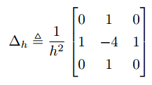
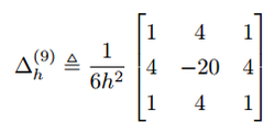
I remember reading long time ago that RE will indeed improve the accuracy of a second-order scheme, increase its convergence order to $O({h^4})$ if implemented properly, but will not produce as accurate results as a scheme that is fourth-order accurate ($O({h^4})$ truncation error) by design. I had seen examples of this in 1D, but I hadn't seen results for 2D so I thought I'd do this test. Let's imagine for now that grid points are uniformly spaced, as was indeed the case in this test. The second-order scheme used is the standard 5-point stencil and the fourth-order scheme is the fantastic 9-point compact stencil.
RE implementation
RE implementation
The RE solution is a linear combination of two solutions calculated on two different grids (representing the solution on two different sets of discrete points, or nodes if you prefer). In order to combine the two solutions we need to have them at the same locations, so if there's no common set of points we then need to somehow bring/project one solution onto the grid of the other. So we need to interpolate. Usually people will perform RE by combining the solution on a grid with say N steps in each dimension (h=1/N), with that on a grid with half or double the spacing h. This way there's no need to use interpolation if we're projecting our final RE result on the coarser grid, because the finer grid already has the solution on all the coarser grid's points. If we want the RE results "printed" on the finer grid's resolution instead, then we need to interpolate in order to "guess" what the coarser grid's solution is at those extra points that the finer grid has. In the 2D case this means we would need to produce N$\times$N values based on information from only 25% as many (the 0.5$\times$0.5$\times$N$\times$N values of our coarse grid).
I prefer keeping the two grid resolutions closer to each other. Too close is not good either though because then the two solutions are not "distinct" enough and the extrapolation loses accuracy. My tests here showed that a spacing ratio of 0.85 is about right. In this case when we interpolate the results of the coarser (0.85$\times$0.85$\times$N$\times$N) grid "upwards", we generate our N$\times$N values now using 72% as many values, as opposed to 25% in the half spacing case. We now definitely need to interpolate of course because the two grids' sets of points are going to be distinct. Simple (2D) local polynomial interpolation was used here. The important detail is that the interpolating polynomial accuracy (degree) needs to be the same or higher than that which we expect to obtain from the extrapolation. I used sixth-degree polynomials for the results in the graph below. That worked fine because the combination of the smoothly-varying field and the high grid resolutions meant that any 7 contiguous points used to fit the polynomials were always pretty much on a straight line. When the function we are trying to find a solution for is less benign, using such high-order polynomials will in general make things worse due to Runge's phenomenon. We would then need to cramp many more grid points in order to avoid this problem. In practice, non-uniform grids are often used anyway in order to properly resolve areas of steep gradients by concentrating more points there, regardless of whether we plan to extrapolate or not.
I prefer keeping the two grid resolutions closer to each other. Too close is not good either though because then the two solutions are not "distinct" enough and the extrapolation loses accuracy. My tests here showed that a spacing ratio of 0.85 is about right. In this case when we interpolate the results of the coarser (0.85$\times$0.85$\times$N$\times$N) grid "upwards", we generate our N$\times$N values now using 72% as many values, as opposed to 25% in the half spacing case. We now definitely need to interpolate of course because the two grids' sets of points are going to be distinct. Simple (2D) local polynomial interpolation was used here. The important detail is that the interpolating polynomial accuracy (degree) needs to be the same or higher than that which we expect to obtain from the extrapolation. I used sixth-degree polynomials for the results in the graph below. That worked fine because the combination of the smoothly-varying field and the high grid resolutions meant that any 7 contiguous points used to fit the polynomials were always pretty much on a straight line. When the function we are trying to find a solution for is less benign, using such high-order polynomials will in general make things worse due to Runge's phenomenon. We would then need to cramp many more grid points in order to avoid this problem. In practice, non-uniform grids are often used anyway in order to properly resolve areas of steep gradients by concentrating more points there, regardless of whether we plan to extrapolate or not.
Results
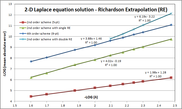
So here's the graph I was talking about. It shows how the average absolute error (across all solution grid points) falls as we make the grid spacing h smaller. Well not exactly all grid points. I've actually excluded the first 5% from the top side of the square domain downwards. The reason is that due to the singularities in the top two corners (the boundary conditions there change discontinuously from unit at the top to zero at the sides), the solution in their vicinity misbehaves. Here we don't care about that so in order to get a clean picture of the orders of convergence under "normal" circumstances, I left those points out of the average error calculation. So on to the results. Expectations were generally confirmed, or even exceeded in the case of the double RE. The latter basically combines two (fourth-order) RE results to extrapolate to a theoretically sixth-order accurate result. With double RE being an extrapolation based on other (single RE) extrapolations (all of which based on interpolations!), I was not sure at all I'd get anywhere near sixth-order. But sure enough, $O({h^{6+}})$ was obtained for this smooth field. As expected, even though the single RE actually achieved slightly better order of convergence than the native fourth-order 9-point scheme in this case, the actual error it produced was significantly higher, about 22 times higher to be exact for the range of h used. The double RE though managed to beat the fourth-order scheme for actual accuracy achieved, producing lower errors when the grid is reasonably fine (for h < 0.01 roughly).


 RSS Feed