OK, so that's not strictly true, I lied to get your attention. You are presumably still interested in either TARF's, finite differences, or AI and I have some original research here for you, so keep reading!
ChatGPT of course is not quite there yet and will likely not be any time soon since this is a specialized application for which code is never public. But we can train our own "AI" to learn the FD engine's behavior and then use it to optimally set it up. More specifically, I am going to train it so that it can propose the optimal grid (or mesh if you prefer) construction for each pricing case (contract and market data).
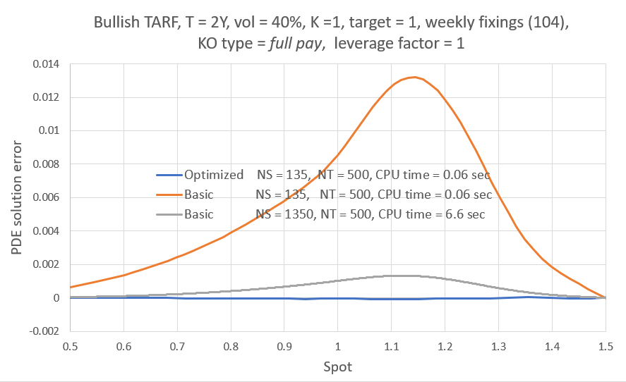
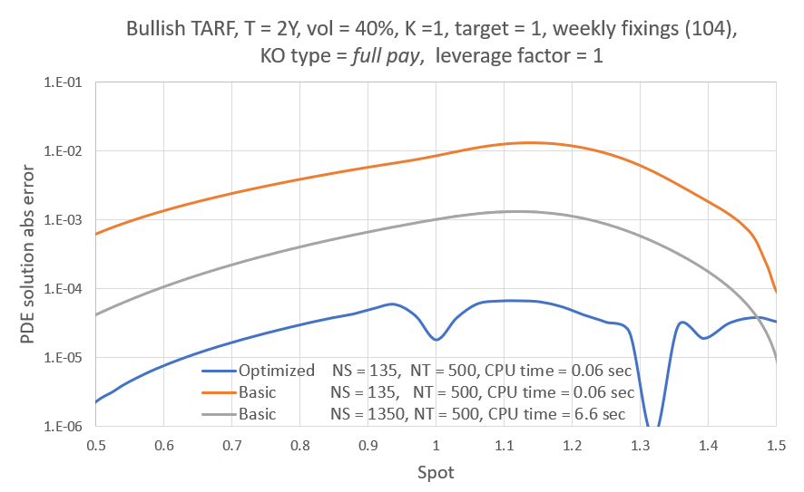
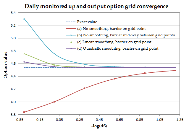
It is in general more computationally efficient to use non-uniform grids that are denser near some point of interest, so that the solution is better resolved there (and less resolved in other areas where we don't care for). In option pricing that can be for example the strike, a barrier, or the spot. This makes the implementation slightly more involved but we can get more accuracy than with uniform grids for the same computational cost, or equivalently the same accuracy for lower cost. This is not a one-size-fits-all solution though. Different problems benefit from different degrees of non-uniformity, as well as choice of focus/cluster point(s) and one does not know a priori how to make these choices optimally. Not only that, some choices may lead to worse accuracy than what we would get using a uniform grid! And this is something that I have always found somewhat frustrating, using a more sophisticated tool with higher inherent accuracy without the ability to "calibrate" it.
But this is 2023 and AI can do almost everything, right? Of course some fear that it will destroy humanity. Others just see it as the new thing that will get them jobs or promotions. Me being naturally curious I had to look into it and at least have some first hand experience. Can it provide me with the (near-)optimal-grid picking tool I've been missing? Actually this is an idea I have meant to try out since I got interested in Neural Networks (NN's) a few years ago. It sounds good because it aims to enhance the traditional method without sacrificing mathematical transparency. After all we are only using the NN to decide on the grid, which we would otherwise do so more or less arbitrarily anyway. We just have to make sure that we let it choose from the range of options that we would and we are safe. As far as I am aware, this particular way of involving NN's in the solution of a PDE is novel, so I am trying out an oiginal idea here.
Now depending on the product to be priced, the grid construction may be simple or more complex. For example it may involve different segments and/or have to make sure certain values are represented by grid points. In my case the grid construction is key to the overall accuracy/efficiency of the engine. I am not going to get into the details here, but it does try to place points on the strike, the underlying level that would meet the remaining target and the spot (the latter only when it doesn''t result in too much stretching). Remember, the grid I am talking about here is the S-grid (i.e. the underlying, here some FX rate) that the 1-D solvers use (please see the first post in this series for a little bit more about the engine). The spacing between the accrued amount (A) planes to which each solver corresponds is also somehow derived from the S-grid. Despite this rather convoluted construction, at the heart of it the S-grid is based on the following well known stretching function:
ChatGPT of course is not quite there yet and will likely not be any time soon since this is a specialized application for which code is never public. But we can train our own "AI" to learn the FD engine's behavior and then use it to optimally set it up. More specifically, I am going to train it so that it can propose the optimal grid (or mesh if you prefer) construction for each pricing case (contract and market data).
It is in general more computationally efficient to use non-uniform grids that are denser near some point of interest, so that the solution is better resolved there (and less resolved in other areas where we don't care for). In option pricing that can be for example the strike, a barrier, or the spot. This makes the implementation slightly more involved but we can get more accuracy than with uniform grids for the same computational cost, or equivalently the same accuracy for lower cost. This is not a one-size-fits-all solution though. Different problems benefit from different degrees of non-uniformity, as well as choice of focus/cluster point(s) and one does not know a priori how to make these choices optimally. Not only that, some choices may lead to worse accuracy than what we would get using a uniform grid! And this is something that I have always found somewhat frustrating, using a more sophisticated tool with higher inherent accuracy without the ability to "calibrate" it.
But this is 2023 and AI can do almost everything, right? Of course some fear that it will destroy humanity. Others just see it as the new thing that will get them jobs or promotions. Me being naturally curious I had to look into it and at least have some first hand experience. Can it provide me with the (near-)optimal-grid picking tool I've been missing? Actually this is an idea I have meant to try out since I got interested in Neural Networks (NN's) a few years ago. It sounds good because it aims to enhance the traditional method without sacrificing mathematical transparency. After all we are only using the NN to decide on the grid, which we would otherwise do so more or less arbitrarily anyway. We just have to make sure that we let it choose from the range of options that we would and we are safe. As far as I am aware, this particular way of involving NN's in the solution of a PDE is novel, so I am trying out an oiginal idea here.
Now depending on the product to be priced, the grid construction may be simple or more complex. For example it may involve different segments and/or have to make sure certain values are represented by grid points. In my case the grid construction is key to the overall accuracy/efficiency of the engine. I am not going to get into the details here, but it does try to place points on the strike, the underlying level that would meet the remaining target and the spot (the latter only when it doesn''t result in too much stretching). Remember, the grid I am talking about here is the S-grid (i.e. the underlying, here some FX rate) that the 1-D solvers use (please see the first post in this series for a little bit more about the engine). The spacing between the accrued amount (A) planes to which each solver corresponds is also somehow derived from the S-grid. Despite this rather convoluted construction, at the heart of it the S-grid is based on the following well known stretching function:
$ S_i=S_{min}+K\left(1+sinh\left(b(\frac{i}{NS}-a)\right)/sinh(ab)\right)$
where K is the clustering point, NS the number of grid spacings and a, b are free parameters. b in particular controls the degree of non-uniformity and is the one we want to be able to choose optimally (as well as K) ; given b and K, a can then be determined so that the grid goes up to $ S_{max}$ (if interested see (1) for more details on employing such a grid).
The main idea:
We want to train a simple Artificial Neural Network (a Multilayer Perceptron) to "learn" the discretization error of the PDE numerical solution as a function of the PDE coefficients, initial and boundary conditions, plus some parameter(s) that drive the grid construction. Once we have a good (and very fast) NN approximation of the error, we can use it to solve for the grid parameters that would minimize it. So we can decide on the optimal grid construction before the actual numerical solution.
In this case, I have a PDE engine that solves for the fair value of an FX TARF contract. So the inputs to the functional of the output (the discretization error, from now on simply referred to as the "error") are the contract details, the market data, the parameter b of the grid stretching function and the clustering point K. Regarding the latter, in some cases it is preferable (meaning the solution error at S = spot, which is where we want the contract value, is lower) to focus the grid on the strike and in others on the spot. By the way, this whole grid selection process will take a fraction of a millisecond, so the added CPU cost will be negligible compared to the actual numerical solution which can take up to a second or more in the worst cases.
The goal here is to get more out of an existing solver. In practice one normally decides on some grid resolution (number of grid spacings in each dimension), so that the average error across all pricings is acceptably low. Remember this is a (pseudo) 2-D solver, we also have the accrued amount (A) planes grid. The number of planes NA will logically be proportional to NS, so the CPU time scales with ${NS^{2}}$. The discretization scheme will typically be second order accurate (in both space and time), so the error scales with $1/{NS^{2}}$, which means it is inversely proportional to the CPU time. So if enabling optimal grid selection can cut the average error of our current set-up in half, we should in theory be able to lower the resolution and get the same accuracy as our current set-up at half the CPU cost.
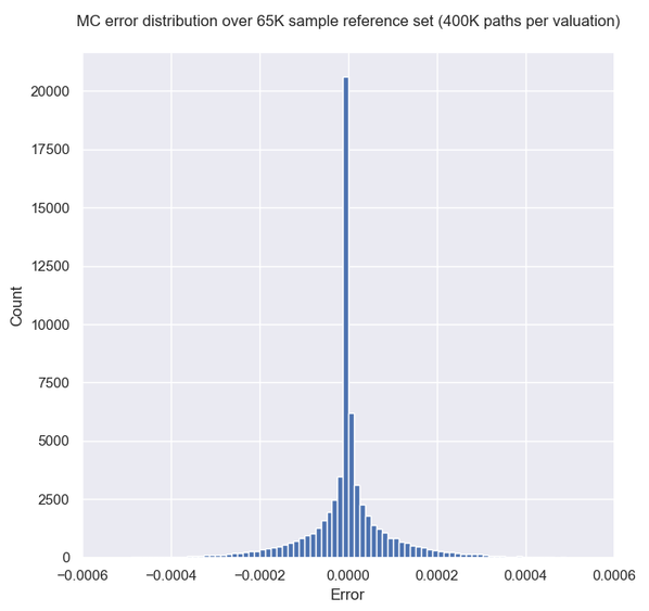
The error refers to some fixed working resolution (here NS=200) and it is calculated as follows: The PDE engine yields the TARF value on the grid points from which we find the value at the current spot $V_{Spot}^{NS=200}$either directly (if there is a grid point on the spot), or otherwise via $4^{th}$ order polynomial interpolation. We then repeat the valuation using a much finer (NS=900) grid (where the solution should be almost grid-converged) to find $V_{Spot}^{Ref}$. The error is then simply $\mid V_{Spot}^{Ref}-V_{Spot}^{NS=200} \mid $. For the reference valuation, K and b were chosen using a heuristic strategy I had in place for my previous two posts. Finally, I used a uniform time grid with NT=250 spacings/year for all valuations here, so the error has a temporal discretization component as well. Here though we are only focusing on fine-tuning the non-uniform "spatial" grid.
The error refers to some fixed working resolution (here NS=200) and it is calculated as follows: The PDE engine yields the TARF value on the grid points from which we find the value at the current spot $V_{Spot}^{NS=200}$either directly (if there is a grid point on the spot), or otherwise via $4^{th}$ order polynomial interpolation. We then repeat the valuation using a much finer (NS=900) grid (where the solution should be almost grid-converged) to find $V_{Spot}^{Ref}$. The error is then simply $\mid V_{Spot}^{Ref}-V_{Spot}^{NS=200} \mid $. For the reference valuation, K and b were chosen using a heuristic strategy I had in place for my previous two posts. Finally, I used a uniform time grid with NT=250 spacings/year for all valuations here, so the error has a temporal discretization component as well. Here though we are only focusing on fine-tuning the non-uniform "spatial" grid.
The Neural Network
I trained a small MLP (4 x 80 hidden layers) with a total of 524K samples, i.e. pairs of input vectors and output ( the error). The inputs and their considered ranges/possible values are shown below. Of course I also created a separate (smaller) test set to monitor the performance of the NN while training it. The inputs for both training and test sets were sampled uniformly from their respective ranges (either continuously or discretely where applicable), with the exception of the spot (lognormal).
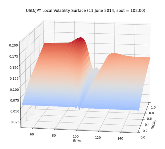
Note that I have switched from using the local volatility model in the previous post, back to constant (BS) volatility here. The reason is just to facilitate my training, since otherwise I would have needed to create (valid) random volatility surfaces and I didn't want to go there for the purposes of this post. It is my view that this wouldn't have been significantly more difficult (if you have the machinery to generate random volatility surfaces at hand). As mentioned in the previous post, the pricing CPU time is the same and I fully expect the NN to be able to capture the error behavior in that case just as well as it does here for constant volatility. Something for the future perhaps.
Note that I have switched from using the local volatility model in the previous post, back to constant (BS) volatility here. The reason is just to facilitate my training, since otherwise I would have needed to create (valid) random volatility surfaces and I didn't want to go there for the purposes of this post. It is my view that this wouldn't have been significantly more difficult (if you have the machinery to generate random volatility surfaces at hand). As mentioned in the previous post, the pricing CPU time is the same and I fully expect the NN to be able to capture the error behavior in that case just as well as it does here for constant volatility. Something for the future perhaps.
| DNN Input parameters | |
| T (yrs) | 0.001 - 2.5 |
| target / strike | 0.0001 - 1 |
| leverage factor | 0, 1, 2 |
| KO type | 0, 1, 2 (No pay, capped pay, full pay) |
| trade direction | 0, 1 (bullish, bearish) |
| num. fixings | weekly or montly freq., remaining fixings follow from T |
| volatility | 2% - 50% |
| spot / strike | lognormal (0, vol * sqrt(T)) |
| rd | -1% - 10% |
| rf | -1% - 10% |
| b (grid non-unidormity) | 1.5 - 15 |
| K (grid cluster point) | 0, 1 (strike, spot) |
By the way, a value b = 1.5 results in a near-uniform grid, while b = 15 makes the grid highly non-uniform (too much actually), with density around the cluster point about 2-3 orders of magnitude higher than at the grid end points.
Usage
So how would we use the trained NN? Given a particular trade and set of market data, we now have a (hopefully) good enough approximation of our PDE engine's expected discretization error as a function of the two grid parameters, i.e. error = f(K, b). We can then proceed to find (K, b) that minimizes f. Normally f(spot, b) and f(strike, b) are convex with a unique minimum. So we could use a method like Brent to find the minimum. But since the NN approximation will be imperfect and may potentially in cases have some spurious local minimum forming somewhere, it is better to just sample the error at m equidistant values in the b-range. I used m = 15 here, first for K = strike and then for K = spot and picked the case with the overall lowest error. This means a total of 30 NN evaluations (inferences), each taking about 0.01ms on a modern CPU core (a few matrix multiplications), so the total prediction of the optimal grid parameters comes at about 0.3-0.4 milliseconds.
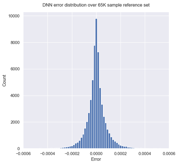
It is worth noting that while we obviously aim to approximate the error functional as closely as possible with the NN, in the end what we really care about is the location of the minimum and not the exact value. So while during training we evaluate the network performance using a metric like MAE or RMSE (note, we are talking about mean (NN approximation) error of the (PDE discretization) error here!), this is not our ultimate test of success. That would be whether the NN really choses the optimal grid construction for the particular trade and market data. To confirm that we would have to solve every case using all possible (K, b) combinations and calculate the actual error against the reference price, which is of course impractical.
In reality the NN will miss the actual minimum in many cases. This is because f(K,b) can be a noisy function and the NN can only smooth it out, in which case it will miss the "fine detail" (more on this below). And even when it is smooth, the approximation may not be accurate enough to point to the correct minimum location. But it doesn't have to be, it just needs to be fairly close. That would be good enough since a close to optimal (K,b) will still beat some arbitrary choice and thus improve on the current strategy (likely some case-agnostic, static grid construction, i.e. using some fixed (K, b) for everything).
Results
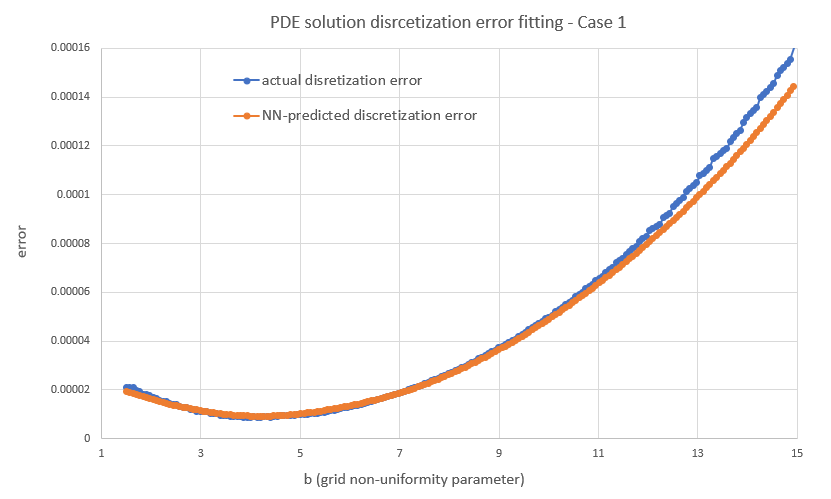
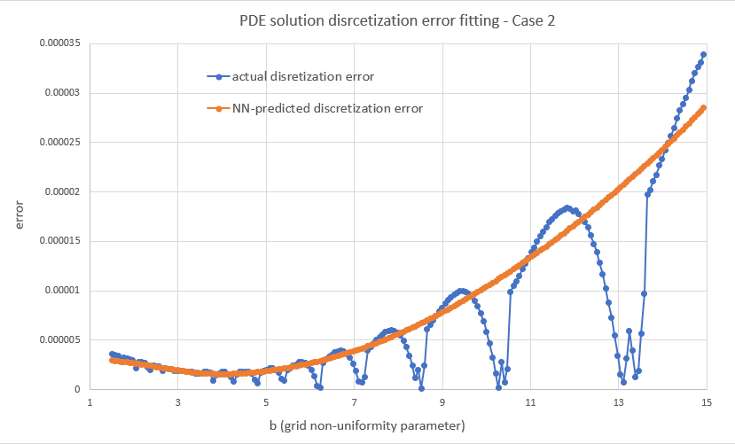
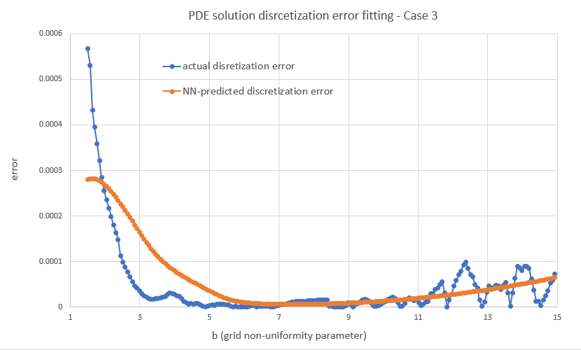
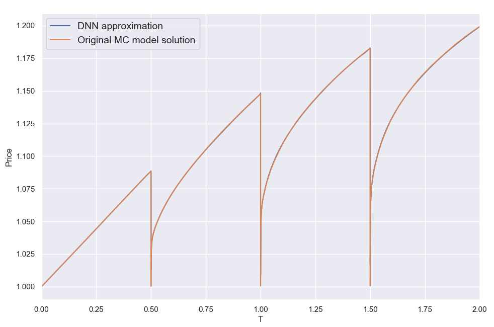
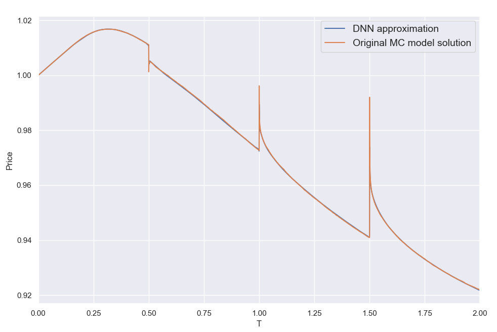
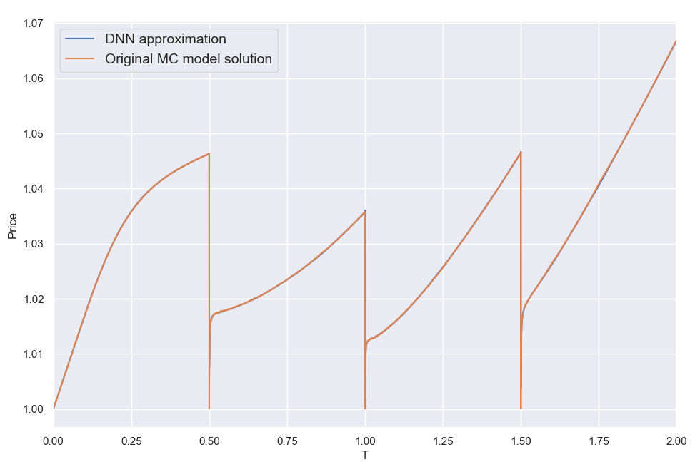
Let's have a look first at some types of error behavior and the resulting NN fits to illustrate what I was referring to above, i.e. the error can be a smooth function of b like in case 1, but it may also look "weird" like the next two cases. As can be seen, the NN smooths out any "high fequency" detail, but correctly locates the level of b where the error would overall be lower. K = Strike here for all three cases.
Overall I found that the NN is able to do a decent job of mapping the error to the inputs, despite its small size. My short testing (I am a freelance at this time with limited resources) indicates that both network and training set sizes used are already producing diminishing returns and in fact I got almost the same benefit training with just half the training set. With slightly larger NN sizes, visual inspection (like the ones above) for a few valuations I've looked into, showed improved fits but that did not translate to significant further improvement in the test below.
So finally to check if all this actually makes the TARF pricing significantly more accurate, I created a test set of 50K random trade & market data scenarios drawn from the same input ranges and distributions I used for the training and calculated the reference prices. I then calculated the prices with the working resolution of NS=200 using grids with various static (K, b) choices, a strike-clustered grid with dynamic NN-proposed optimal b and finally a fully NN-powered grid, with both the clustering focus and the value of b chosen by the NN dynamically (on a trade & market data basis). And then calculated the mean absolute error (MAE) across the test set for each of these strategies. The average pricing time with the working resolution (on a single CPU core) was 0.27 secs and the longest about 1.5 secs.
Table 1. Effect of different finite difference grid constructions on the accuracy of FX TARF valuations (mean absolute discretization error (for NS = 200) across 50,000 random trade & market data scenarios).
| Grid focus (K) | b | Test set MAE |
| Strike | 4 | 4.4E-06 |
| 5 | 2.2E-06 | |
| 6 | 1.6E-06 | |
| 7 | 1.7E-06 | |
| 8 | 2.7E-06 | |
| 9 | 4.6E-06 | |
| Spot | 4 | 3.2E-05 |
| 5 | 2.6E-05 | |
| 6 | 3.8E-05 | |
| Strike | NN proposed | 7.0E-07 |
| NN proposed | NN proposed | 4.0E-07 |
| Heuristic | Heuristic | 1.8E-06 |
As can be seen, using the strike as the grid focal point is generally the better "static "choice here, producing on average about an order of magnitude lower errors than when using the spot. The fixed value of b that minimizes the average error seems to be around b = 6. So if we were to just pick a simple grid construction strategy, this would be it, (K = Strike, b = 6). We then see that sticking with K = Strike and letting the NN pick the optimal value of b for each scenario, cuts the error by more than half. So pretty good I thought, but I knew that there are cases where K = Spot is a better choice. So could the NN successfully recognize such cases (or at least most of them) and switch to targeting the spot for those? The answer seems to be yes; letting the NN pick the optimal K as well, almost halves the error yet again.
Table 2. Comparison of the best static grid construction strategy with the optimal (NN-powered) strategy. Accuracy of FX TARF valuations (spatial discretization error for NS = 200) across 50,000 random trade & market data scenarios.
| (K=Strike, b=6) | NN proposed (K, b) | |
| MAE | 1.6E-06 | 4.0E-07 |
| RMSE | 2.3E-05 | 1.8E-06 |
| Cases with error > 1.E-04 | 92 | - |
| Maximum error | 2.3E-03 | 8.6E-05 |
Not only that but it also drastically reduces large errors, the maximum error being < 1 b.p. while the best static grid strategy produces errors of up to 23 b.p. and has 92 scenarios priced with error > 1b.p. Or in terms of RMSE, the NN fine-tuning of the finite difference grid reduces the pricing RMSE by a factor of 12. Out of curiosity I also included in the test the (heuristic) construction I was using before and surprisingly it was a bit worse than the best simple construction. Oh well (it was a bit better at reducing large errors though).
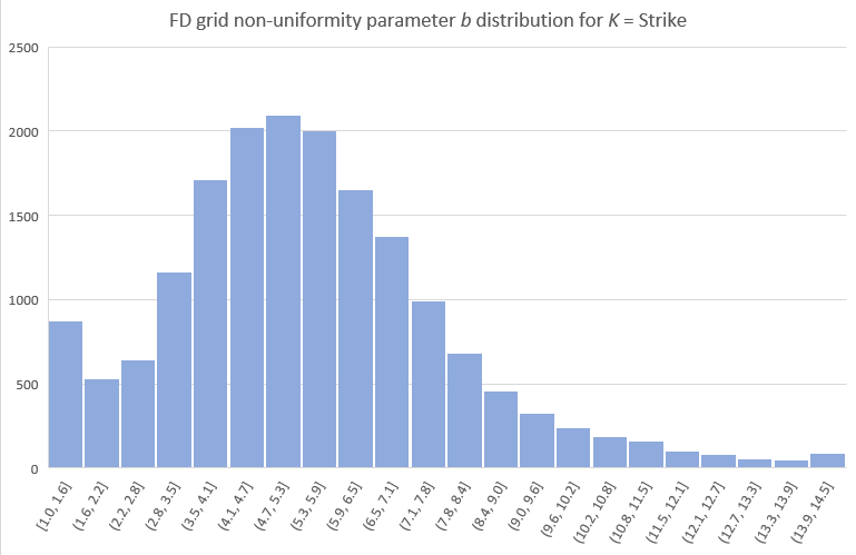
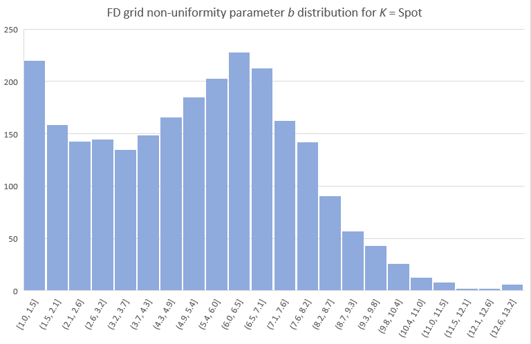
There is of course a lot of other interesting details (figures, tables) I could include, but I will stop here with the b distributions chosen by the NN for the test set, separately for K = Strike and K = Spot cases. Note that in some cases (mostly when the spot is the preferred grid focal point) a close to uniform grid is indeed optimal. The NN opted to use K = Spot for about 12% of the cases.
Before concluding I should probably stress that the NN is specifically trained to approximate the discretization error for a particular grid resolution (here NS=200) and if used to fine-tune the construction of a grid with a different number of spacings, the result will not in general be optimal. It will though very likely still improve on the best static construction. As a quick test I repriced the 50K test scenarios but this time with NS=100 grids, using the best static choice of (K = Strike, b = 6) plus the NN proposed (K, b) and calculated the errors like before. The NN-assisted construction still managed to cut the test MAE of the static construction to less than half (but not quite by a factor of 4 as it did for NS=200). To get the full benefit we would naturally need to train an NN specifically for NS=100.
Conclusion
So it turns out that training a small ANN to pick the optimal (trade & market data specific) finite difference grid construction for each pricing case, works and reduces discretization error levels significantly. This of course means that we could switch to smaller grid sizes, thus saving a lot of CPU time and resources.
Note that I went straight to applying this idea to a rather involved, "real world" PDE solver (with a less than straightforward grid generation), instead of trying it out first on a more "academic" test problem, say a simple barrier option. I may still do that out of curiosity.
Another potential variation would be to also include the resolution NS in the training, so that we can then be able to pick the best (NS, K, b) strategy for a desired error level.
Thanks for reading. If you found this idea interesting and decide to use it in your own research/work, please acknowledge this article and do get in touch, it would be nice to hear from you.
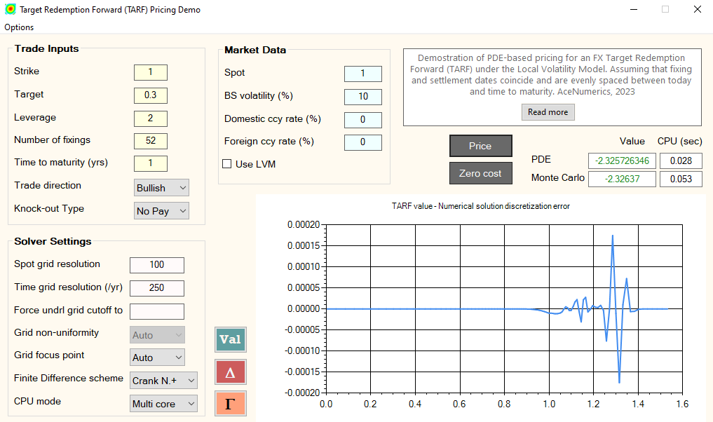
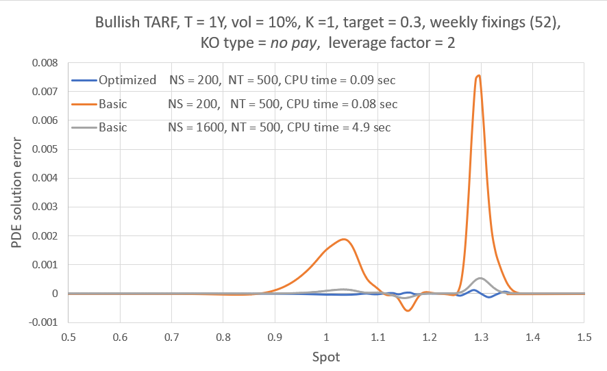
Finally, a demo TARF pricing GUI showcasing the overall speed of the PDE engine, and the effectiveness of the present "smart" grid construction in particular, is available for anyone interested.
Note that I went straight to applying this idea to a rather involved, "real world" PDE solver (with a less than straightforward grid generation), instead of trying it out first on a more "academic" test problem, say a simple barrier option. I may still do that out of curiosity.
Another potential variation would be to also include the resolution NS in the training, so that we can then be able to pick the best (NS, K, b) strategy for a desired error level.
Thanks for reading. If you found this idea interesting and decide to use it in your own research/work, please acknowledge this article and do get in touch, it would be nice to hear from you.
Finally, a demo TARF pricing GUI showcasing the overall speed of the PDE engine, and the effectiveness of the present "smart" grid construction in particular, is available for anyone interested.
Yiannis Papadopoulos, Zurich, November 2023
 RSS Feed