It well known that pure diffusion stochastic volatility (SV) models like Heston struggle to reproduce the steep smiles observed in the implied volatilities of short-term index options. Trying to remedy this deficiency, the usual approach is to introduce jumps. More recently and as an alternative to jumps, some researchers have been experimenting with the use of fractional Brownian motion as the driver for the volatility process. Volatility they say is rough. Such a model is apparently able to capture steep short-term smiles. Basically both these approaches assume that pure diffusion models are not up to the task so alternatives are needed.
However, other voices suggest that this isn't necessarily true and that models of the Heston type have simply not been used to their full potential. They say why use a deterministic starting point $v_0$ for the variance when the process is really hidden and stochastic? Instead, they propose to give such traditional SV models a "hot start", that is assume that the variance today is given by some distribution and not a fixed value. Mechkov [1] shows that when the Heston model is used like that it is indeed capable of "exploding" smiles as expiries tend to zero. Jacquier & Shi [2] present a study of the effect of the assumed initial distribution type.
The idea seems elegant and it's the kind of "trick" I like, because it's simple to apply to an existing solver so it doesn't hurt trying it out. And it gets particularly straightforward when the option price is found through a PDE solution. Then the solution is automatically returned for the whole range of possible initial variance values (corresponding to the finite difference grid in the v-direction). So all one has to do in order to find the "hot-started" option price at some asset spot $ S_0 $ is average the solution across the $ S=S_0 $ grid line using the assumed distribution. Very simple. Of course we have to choose the initial distribution family-type and then we can find the specific parameters of that distribution that best fit our data. How? We can include them in the calibration.
So here I'm going to try this out on a calibration to a chain of SPX options to see what it does. But why limit ourselves to Heston? Because it has a fast semi-analytical solution for vanillas you say. I say I can use a fast and accurate PDE solver instead, like the one I briefly tested in my previous post. Furthermore, is there any reason to believe that a square root diffusion specification for the variance should fit the market, or describe its dynamics better? Maybe linear diffusion could work best, or something in between. The PDE solver allows us to use any variance power p for the diffusion coefficient between 0.5 and 1, so why not let the calibration decide the optimal p, together with the initial distribution parameters and the other model parameters. Let's call this the Randomized Optimal Diffusion (ROD) SV "model".
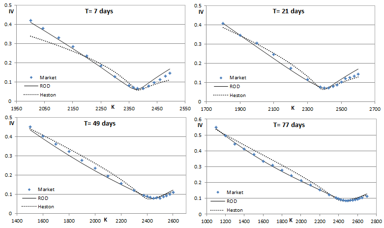
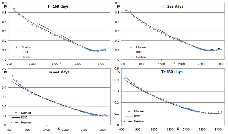
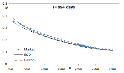
Sounds complicated? It actually worked on the first try. Here's what I got for the end of Q1 2017. Just using the PDE engine and Excel's solver for the optimization. The calibration involved 262 options of 9 different expiries ranging from 1W to 3Y and took a few minutes to complete. If one restricts the calibration to mainly short-term expiries then better results are obtained, but I wanted to see the overall fit when very short and long expiries are fitted simultaneously. I am also showing how the plain Heston model fares. Which on the face of it is not bad, apart for the very short (1W) smile. Visually what it does is try to "wiggle its way" into matching the short-term smiles. The wiggle seems perfectly set up for the 3W smile, but then it turns out excessive for the other expiries. The ROD model on the other hand avoids excessive "wiggling" and still manages to capture the steep smiles of the short expiries pretty well. The optimal model power p here was found to be 0.84. This is responsible for the less wiggly behavior compared to Heston's p = 0.5. The ability to capture the steep short-term smiles is solely due to the hot-start. And it's the hot-start that "allows" for that higher p. To put it another way, by making it easy to fit the short-term smiles it then allows for a better fit for all expiries. The overall RMSE for the Heston model is 1.56% while for the ROD model it's 0.86%.
But the RMSE only tells half the story. The Feller ratio corresponding to Heston's fitted parameters is 0.09, which basically means that the by far most probable (risk-neutral) long-run volatility value is zero. In other words, the assumed volatility distribution is not plausible. The randomization idea is neither without any issues, despite the impressive improvement in fit. The optimizer calibrated to a correlation coefficient of -1 for this experiment, which seems extreme and not quite realistic.
However, other voices suggest that this isn't necessarily true and that models of the Heston type have simply not been used to their full potential. They say why use a deterministic starting point $v_0$ for the variance when the process is really hidden and stochastic? Instead, they propose to give such traditional SV models a "hot start", that is assume that the variance today is given by some distribution and not a fixed value. Mechkov [1] shows that when the Heston model is used like that it is indeed capable of "exploding" smiles as expiries tend to zero. Jacquier & Shi [2] present a study of the effect of the assumed initial distribution type.
The idea seems elegant and it's the kind of "trick" I like, because it's simple to apply to an existing solver so it doesn't hurt trying it out. And it gets particularly straightforward when the option price is found through a PDE solution. Then the solution is automatically returned for the whole range of possible initial variance values (corresponding to the finite difference grid in the v-direction). So all one has to do in order to find the "hot-started" option price at some asset spot $ S_0 $ is average the solution across the $ S=S_0 $ grid line using the assumed distribution. Very simple. Of course we have to choose the initial distribution family-type and then we can find the specific parameters of that distribution that best fit our data. How? We can include them in the calibration.
So here I'm going to try this out on a calibration to a chain of SPX options to see what it does. But why limit ourselves to Heston? Because it has a fast semi-analytical solution for vanillas you say. I say I can use a fast and accurate PDE solver instead, like the one I briefly tested in my previous post. Furthermore, is there any reason to believe that a square root diffusion specification for the variance should fit the market, or describe its dynamics better? Maybe linear diffusion could work best, or something in between. The PDE solver allows us to use any variance power p for the diffusion coefficient between 0.5 and 1, so why not let the calibration decide the optimal p, together with the initial distribution parameters and the other model parameters. Let's call this the Randomized Optimal Diffusion (ROD) SV "model".
Sounds complicated? It actually worked on the first try. Here's what I got for the end of Q1 2017. Just using the PDE engine and Excel's solver for the optimization. The calibration involved 262 options of 9 different expiries ranging from 1W to 3Y and took a few minutes to complete. If one restricts the calibration to mainly short-term expiries then better results are obtained, but I wanted to see the overall fit when very short and long expiries are fitted simultaneously. I am also showing how the plain Heston model fares. Which on the face of it is not bad, apart for the very short (1W) smile. Visually what it does is try to "wiggle its way" into matching the short-term smiles. The wiggle seems perfectly set up for the 3W smile, but then it turns out excessive for the other expiries. The ROD model on the other hand avoids excessive "wiggling" and still manages to capture the steep smiles of the short expiries pretty well. The optimal model power p here was found to be 0.84. This is responsible for the less wiggly behavior compared to Heston's p = 0.5. The ability to capture the steep short-term smiles is solely due to the hot-start. And it's the hot-start that "allows" for that higher p. To put it another way, by making it easy to fit the short-term smiles it then allows for a better fit for all expiries. The overall RMSE for the Heston model is 1.56% while for the ROD model it's 0.86%.
But the RMSE only tells half the story. The Feller ratio corresponding to Heston's fitted parameters is 0.09, which basically means that the by far most probable (risk-neutral) long-run volatility value is zero. In other words, the assumed volatility distribution is not plausible. The randomization idea is neither without any issues, despite the impressive improvement in fit. The optimizer calibrated to a correlation coefficient of -1 for this experiment, which seems extreme and not quite realistic.
By the way, this experiment is part of some research I've been doing in collaboration with Alan Lewis, the results of which will be available/published soon.
 RSS Feed