My old option pricer (which you can download "refurbished" here) had a basic stochastic volatility (Heston) solver which never really passed the testing phase, so I kept it hidden. Besides, it was using SOR to solve the full system at each time-step, so it can't compete with the modern "state of the art" ADI variants. Or can it?
Well I decided to give it another try and see how it compares really after a few optimizing tweaks.
The Heston Partial Differential Equation
We are trying to solve the following PDE by discretizing it with the finite difference method:
$$\frac{\partial V}{\partial t} = \frac{1}{2} S^2 \nu\frac{\partial^2 V}{\partial S^2}+\rho \sigma S \nu \frac{\partial^2 V}{\partial S \partial \nu} + \frac{1}{2}\sigma^2\nu\frac{\partial^2 V}{\partial \nu^2} + (r_d-r_f)S \frac{\partial V}{\partial S}+ \kappa (\eta-\nu) \frac{\partial V}{\partial \nu}-r_d V $$
where $\nu$ is the variance of the underlying asset $S$ returns, $\sigma$ is the volatility of the $\nu$ process, $\rho$ the correlation between the $S$ and $ \nu$ processes and $\eta$ is the long-term variance to which $\nu$ is mean-reverting with rate $\kappa$. Here $S$ follows geometrical Brownian motion and $\nu$ the CIR (Cox, Ingersoll and Ross) mean-reverting process.
Time-discretization: Four-level fully implicit (4LFI, or FI-BDF3)
After we discretize the PDE we are left with an algebraic system of equations relating the values at each grid point (i,j) with those at its neighboring points. With the standard implicit scheme (Euler) the values at time n+1 are found as $ V_{i,j}^{(n+1)} = (B \cdot dt+V_{i,j}^{(n)})/(1-a_{i,j} \cdot dt) $ for each grid point (i,j). $B$ is a linear combination of $ V^{(n+1)} $ at (i,j)'s neighboring points and $a_{i,j}$ the coefficient of $ V_{i,j} $ arising from the spatial discretization. So we need to solve the system of unknowns $ V_{i,j}^{(n+1)} $.
The 3LFI (otherwise known as implicit BDF2) scheme just adds a little information from time point n-1 and can simply be described as: $ V_{i,j}^{(n+1)} = (B \cdot dt+2 \cdot V_{i,j}^{(n)}-0.5 \cdot V_{i,j}^{(n-1)})/(1.5-a_{i,j} \cdot dt) $, $a_{i,j}$ and $B$ being the same as before. This little addition makes the 3LFI/BDF2 scheme second order in time, whereas the standard implicit is only first order.
This scheme is strongly A-stable (?), so unlike something like Crank-Nicolson (CN) it has built-in oscillation-damping on top of being unconditionally stable. So I tested this first and while it worked pretty well, I found that it produced slightly larger errors than CN. That is while they're both second-order accurate, CN's error-constant was lower. Which is not surprising, central discretizations often produce higher accuracy than their one-sided counterparts of the same order. Moreover it was notably less time-converged compared to the ADI schemes using the same number of time-steps.
So I decided to go for higher-spec. Especially since it comes really cheap in terms of implementation. Adding an extra time-point gives us the 4LFI or BDF3 scheme, which is third order:
$$ BDF3 : \quad V_{i,j}^{(n+1)} = \left (B \cdot dt+3 \cdot V_{i,j}^{(n)}-\frac 3 2 \cdot V_{i,j}^{(n-1)}+\frac 1 3 \cdot V_{i,j}^{(n-2)}\right)/\left(\frac {11} 6 - a_{i,j} \cdot dt\right) \qquad (1)$$
While such a scheme is no longer strictly unconditionally stable (it's almost A-stable), it should still be almost as good as and should preserve the damping qualities of 3LFI/BDF2. As it happens, the results it produces are significantly more accurate than both the 3LFI/BDF2 and the ADI schemes for any number of time-steps. Third order beats second order easily here, despite being a one-sided one. Finally as an added bonus, it adds a little to the diagonal dominance of the iteration matrix of the SOR solver so it helps convergence as well.
Now since this is a multi-step scheme (it needs the values not just from the previous time level but also from two levels before that), we need to use something different for the first couple of time steps, a starting procedure. For the very first step we need a two-level (single step) scheme. We cannot use CN because this will allow spurious oscillations to occur given the non-smooth initial conditions of option payoff functions. Instead one can use the standard Implicit Euler scheme plus local extrapolation: we first use the IE scheme for 4 sub-steps of size dt/4 to get the values $ V_{fine}^1$ at the end of the first time step. We then repeat, this time using 2 sub-steps of size dt/2 to obtain $ V_{coarse}^1$ and get the final composite values for the first time step as $(4V_{fine}^1-V_{coarse}^1)/3 $. For the second time step we just use the 3LFI/BDF2.
Space-discretization and boundary conditions
Central finite differences are used for everything, except again for the v = 0 boundary, where we need to use a one-sided (three-point) upwind second-order discretization for the first v-derivative. Hout & Foulon [1] also use that upwind discretization in some cases where v > 1, but I stick to the central formula here. And of course I make sure that the strike falls in the middle between two grid points, which is something that occasionally people seem to neglect in a few publications I've seen. Suitable Neumann and/or Dirichlet boundary conditions are used everywhere except for the v = 0 variance boundary where we require that the PDE itself (with many terms being zero there) is satisfied, all as described in Hout & Foulon [1].
System solver
I used successive over-relaxation (SOR) to solve the resulting system because it's so easy to set up and accommodate early exercise features. On the other hand it is in general quite slow and moreover its speed may depend significantly on the chosen relaxation factor $\omega$. This is where the hand-made part comes in. I am using an SOR variant called TSOR together with a simple algorithm that adjusts $\omega$ as it goes, monitoring proceedings for signs of divergence as well (e.g. residual increasing instead of decreasing). I am not 100% sure my implementation is bug free, but it seems that the resulting SOR iteration matrix is not always such that it leads to convergence. There's a maximum $\omega$ which presumably makes the spectral radius of the iteration matrix less than one, but I've not pursued any further analysis on that, relying instead on the heuristic algorithm to keep it safe and close to optimal. All in all the modifications compared to the standard SOR amount to a few lines of code. I may write details of TSOR in another post but for the moment let's just say that it speeds things up about 3 times compared to standard SOR, plus it seems less dependent on $\omega$.
Compared to Alternating Direction Implicit (ADI) methods
As I mentioned above, I wanted to compare this general purpose, old-school method to what people use nowadays for Heston (and other parabolic PDE's with mixed derivatives), which will usually be an ADI variant like Graig-Sneyd, Modified Graig-Sneyd, or Hundsdorfer-Verwer. To this end I did not implement said methods myself, but I downloaded and used QuantLib which does implement them. It's the first time that I use QuantLib and was pleasantly surprised by the available functionality (but less so by the lack of quantitative-level documentation). So I will be comparing with their implementation.
I will use the following 6 sets of parameters found in the relevant literature in order to make a few quick comparisons:
Table 1. Model parameter sets from literature.
| κ | η | σ | ρ | rd | rf | T | K | νo | Ref | |
| Case 0 | 5 | 0.16 | 0.9 | 0.1 | 0.1 | 0 | 0.25 | 10 | 0.0625 | [2] |
| Case 1 | 1.5 | 0.04 | 0.3 | -0.9 | 0.025 | 0 | 1 | 100 | 0.0625 | [1] |
| Case 2 | 3 | 0.12 | 0.04 | 0.6 | 0.01 | 0.04 | 1 | 100 | 0.09 | [1] |
| Case 3 | 0.6067 | 0.0707 | 0.2928 | -0.7571 | 0.03 | 0 | 3 | 100 | 0.0625 | [1] |
| Case 4 | 2.5 | 0.06 | 0.5 | -0.1 | 0.0507 | 0.0469 | 0.25 | 100 | 0.0625 | [1] |
| Case 5 | 3 | 0.04 | 0.01 | -0.7 | 0.05 | 0 | 0.25 | 100 | 0.09 | [3] |
The first case has been used by Ikonen & Toivanen [2] and other authors, cases 1-4 are from Hout & Foulon [1] and the last one is from Sullivan & Sullivan [3] who quote that such a set would be typical of a calibration of the model to equity market options. Note the very small volatility of variance $ \sigma$ which makes the PDE strongly convection-dominated in the v direction, plus the strongly negative correlation.
So let's start with a very unscientific comparison. Table 2 shows the prices, errors and timings for at-the-money puts at the current variance levels $\nu_o$ of table 1, as calculated by the present solver and the modified Craig-Sneyd ADI scheme in QLib. This is just a quick and dirty way to get a first idea since there are more differences than just the method. QLib discretizes in log(S) while the present implementation is based on the original PDE in S. QLib uses non-uniform grids while for this comparison I used uniform grids. In order to make things as equal as possible I let the grid stretch approximately as far right in S and v as QLib does for each case, though the latter truncates the grid from the left as well while I always start from zero. The boundary conditions are probably different as well.
Finally a fine grid was chosen deliberately since this is where SOR-based solvers are usually reported to suffer the most in terms of efficiency when compared with splitting schemes like ADI. The stopping criterion was set low enough so that the prices are converged to all six digits shown. This is definitely lower than the average discretization error and thus unnecessary, so in real-life situations the present solver could be set up to be a little faster still.
Table 2. Random comparison between QLib's Modified Graig-Sneyd ADI Heston solver using non-uniform grids in log(S), v and the present implementation using uniform grids in S, v, in both cases with 500x250x150 (asset x variance x time) steps. The exact solutions were obtained via a semi-analytical method. Timings are on a i7-920 PC (from 2009).
| Solver | Price | |Error| | CPU secs | |
| Case 0 | Present | 0.501468 | 0.000002 | 4.1 |
| QLib MGS | 0.501469 | 0.000003 | 7.5 | |
| Exact | 0.5014657 | - | - | |
| Case 1 | Present | 7.46150 | 0.000234 | 6.2 |
| QLib MGS | 7.46175 | 0.000015 | 7.5 | |
| Exact | 7.461732 | - | - | |
| Case 2 | Present | 14.4157 | 0.000008 | 7.4 |
| QLib MGS | 14.4166 | 0.000861 | 7.5 | |
| Exact | 14.41569 | - | - | |
| Case 3 | Present | 12.0821 | 0.001076 | 6.6 |
| QLib MGS | 12.0830 | 0.000122 | 7.5 | |
| Exact | 12.08315 | - | - | |
| Case 4 | Present | 4.71629 | 0.000007 | 3.8 |
| QLib MGS | 4.71637 | 0.000072 | 7.5 | |
| Exact | 4.716294 | - | - | |
| Case 5 | Present | 4.83260 | 0.000002 | 4.3 |
| QLib MGS | 4.83267 | 0.000069 | 7.5 | |
| Exact | 4.832600 | - | - |
As I've said above this is really a dirty comparison, but basically I just wanted to see how much slower the present scheme is, is it 3 times, or 5 times, or 10. The next thing to check would be robustness, but I'll leave that for a different post. So then, to my surprise the present method seems to be overall on par speed-wise with the ADI method, faster even for the chosen number of time steps. This is in contrast to what one reads in the literature where SOR is always the "slow" method one uses to compare with the more efficient modern methods. Not the case here with the 4LFI/BDF3 scheme and TSOR. Please note that in getting the above timings the relaxation factor $\omega$ was not chosen experimentally for each case so as to get optimal convergence. Instead it was left to the simple algorithm to adjust it dynamically as the solution progressed (starting from preset rough estimates based on the grid resolution). Execution time differs from case to case as one would expect, given the different characteristics of the iteration matrix for each parameter set, case 2 proving the most challenging. In contrast the ADI scheme's execution times always scale linearly with the grid size regardless of the input parameters.
QLib by default focuses the S-grid density around the strike and this should be optimal at least for the at-the-money valuations done here. I am not sure I understand what it is doing for the v-grid, but somehow it doesn't seem right to me since it doesn't vary smoothly. Maybe I am missing something. Anyway, do the above results indicate that non-uniform grids are not better after all? No. As I've also briefly discussed here, non-uniform grids do of course perform better in general, but their added value really depends on each case and one may well get a more accurate result for a particular spot with a uniform S-grid instead. I think that's what we can take from here. And perhaps that QLib's grid generation is not optimal. Or more generally that non-uniform grids need more care. I should make it clear that these comments apply to the S-grid only, across which the initial conditions are non-smooth/discontinuous. Based on a few preliminary tests I've done, the advantage brought by a non-uniform v-grid may be more predictable but more testing is needed.
A better picture of the quality of the solution is possible if we look at the error distribution across different values of S and v, instead of a single point. Like an error surface, or curve. Figure 1 shows a cross section of the error surface at v = $\eta$ (the long run variance) for case 0. As I mentioned above, I am not sure how the non-uniform v-grid is constructed in QLib, but it definitely is centered on $ \eta$ when the initial variance specified v0 equals $\eta$.
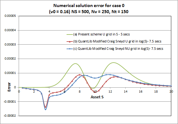
Figure 1. Error distribution for case 0 at v0 = 0.16, for a) the present solver with uniform (U) grids in S and v, b) QuantLib's MGS ADI scheme using non-uniform (NU) grids in log(S) centered on each S point and c) QuantLib's MGS ADI scheme using uniform grids in log(S).
When we price an option by solving a PDE we get the entire solution surface for the grid range S,v where we discretized it. So if we have the exact solution as well (which we do here for European options, courtesy of semi-analytic Fourier methods), we can calculate the error surface. I can readily do that with the present solver, but I could not figure out an easy way to extract the whole solution from QLib. Instead I had to run multiple QLib valuations to get each point in curves (b) and (c) separately. Note that in doing so QLib uses a different S-grid range every time. For curve (b) I forced QLib to use a uniform grid (in log(S) always). For curve (c) I changed QLib's default behaviour (which is to always make the NU grid cluster around the strike regardless of the given asset spot S) and make it cluster around the spot S for which we want to get the option price each time. This should in theory minimize the error for each S point. In contrast, with the present solver we pay no special attention to each S and get the whole curve in one go for all S. I also tried QLib with the NU grid always centered on the strike but that gives much larger errors left of the strike (not shown here). Note that QLib still used NU grids in v for both curves (b) and (c).
So what do we see in this (used frequently in literature) case ? Two things: First that the non-uniform grid construction in log(S) seems to offer no real advantage over the uniform one. If anything in this example the uniform grid performs slightly better and gives lower errors for at-the-money valuations. Second that the uniform grid in S of the present solver gives comparable results, though the QLib average error does seem lower. Remember that QLib uses a much denser v-grid here which of course helps smooth out the error curve. Oh, and by complete fluke the present solver gives zero error at-the-money.
American option pricing
Another advantage of SOR when it comes to option pricing, apart from its simplicity, is the ease with which one can incorporate early exercise features. It's literally one extra line of code (OK, maybe a couple more counting the equally trivial changes in the boundary conditions). So let's have a look at the accuracy of the results produced by the present method. I will again use test case 0 from table 1 which has been used extensively in the literature for American option pricing under Heston (see for example [2]). We should note here that with the ADI schemes there are various ways with which one can handle early exercise. One of the best is probably the operator splitting method of Ikonen & Toivanen in [2], although in that paper they use it with different time-discretizations. I will compare with their results below but first I will again make a quick comparison with QLib's American Heston pricing functionality, using the same ADI scheme (MGS) like before. QLib does not use a "proper" method for handling early exercise, it simply applies the American constraint explicitly, after the prices have been obtained like European at each time step (explicit payoff method). Such an approach cannot give very accurate results. With SOR on the other hand (in this context called PSOR, i.e. Projected SOR) the American constraint is really "blended into" the solution. We apply it every time we update the value of each grid point and the next point we update can "feel" the effect of the previous points we have updated, i.e. it can feel that the values of the previous points have been floored by the payoff. And this is repeated many times (as many as the iterations needed for the solution to converge for that time step), which leads to all the points properly "sharing" what each needs to know about the early exercise effect. So in the end of each time step the PDE and the constraint are satisfied at each point simultaneously. Unlike with the explicit, a posteriori enforcement of the constraint in QLib, which unavoidably cancels all the good work the ADI had done before to exactly satisfy the discretized PDE at each point. The result of these different ways of incorporating early exercise can be seen below.
Another advantage of SOR when it comes to option pricing, apart from its simplicity, is the ease with which one can incorporate early exercise features. It's literally one extra line of code (OK, maybe a couple more counting the equally trivial changes in the boundary conditions). So let's have a look at the accuracy of the results produced by the present method. I will again use test case 0 from table 1 which has been used extensively in the literature for American option pricing under Heston (see for example [2]). We should note here that with the ADI schemes there are various ways with which one can handle early exercise. One of the best is probably the operator splitting method of Ikonen & Toivanen in [2], although in that paper they use it with different time-discretizations. I will compare with their results below but first I will again make a quick comparison with QLib's American Heston pricing functionality, using the same ADI scheme (MGS) like before. QLib does not use a "proper" method for handling early exercise, it simply applies the American constraint explicitly, after the prices have been obtained like European at each time step (explicit payoff method). Such an approach cannot give very accurate results. With SOR on the other hand (in this context called PSOR, i.e. Projected SOR) the American constraint is really "blended into" the solution. We apply it every time we update the value of each grid point and the next point we update can "feel" the effect of the previous points we have updated, i.e. it can feel that the values of the previous points have been floored by the payoff. And this is repeated many times (as many as the iterations needed for the solution to converge for that time step), which leads to all the points properly "sharing" what each needs to know about the early exercise effect. So in the end of each time step the PDE and the constraint are satisfied at each point simultaneously. Unlike with the explicit, a posteriori enforcement of the constraint in QLib, which unavoidably cancels all the good work the ADI had done before to exactly satisfy the discretized PDE at each point. The result of these different ways of incorporating early exercise can be seen below.
Table 3. Temporal convergence for the American (at the money) put of case 0, for the present solver (4LFI/BDF3 with Projected TSOR) and QLib's Modified Graig-Sneyd Heston solver with the explicit payoff (EP) method. NS=200, Nv=100.
| Present solver BDF3 - PTSOR | QLib MGS - EP | |||||
| Nt | Price | |Error| | CPU secs | Price | |Error| | CPU secs |
| 50 | 0.519890 | 0.000004 | 0.33 | 0.519376 | 0.000557 | 0.28 |
| 100 | 0.519893 | 0.000001 | 0.44 | 0.519653 | 0.000280 | 0.51 |
| 200 | 0.519894 | 0.000000 | 0.43 | 0.519793 | 0.000140 | 0.97 |
| 400 | 0.519894 | 0.000000 | 0.73 | 0.519863 | 0.000070 | 1.9 |
| 800 | 0.519894 | 0.000000 | 1.1 | 0.519900 | 0.000033 | 3.7 |
| 1600 | 0.519894 | 0.000000 | 1.6 | 0.519918 | 0.000015 | 7.3 |
| 20000 | 0.519894 | 0 | - | 0.519934 | 0 | - |
Table 3 shows the pricing of the American put of case 0 from table 1 (also used for such tests in [2]) with a fixed spatial grid of 200 x 100 and increasing number of time steps. The time-converged value was calculated in both cases using 20000 time steps. Note that the converged values are not the same for the two solvers because they are using different spatial discretizations.
As we can see, apart from the first order convergence, the explicit payoff method of QLib also comes with a large error constant. Even with 1600 time steps the error is greater than that of the present solver with only 50 time steps. That said, the predictably first order convergence of the Qlib approach means that one can use Richardson extrapolation and get much improved accuracy.
The other thing to note is that the present solver becomes much faster than the ADI when the number of time steps is increased. Unfortunately this proves to be a rather useless advantage since given its high temporal accuracy one would not need to use a large number of time steps anyway.
Ikonen & Toivanen in [2] provide extensive results for the same test case which include the use of the standard (P)SOR with three second order time schemes (Crank-Nicolson, BDF2 and Runge Kutta), as well as their operator splitting (OS) method coupled with a multigrid (MG) solver. Their space discretization is very similar to the one used here (second-order central schemes for first and second derivative terms), although they do add some diffusion in areas of the solution where convection dominates, in order to avoid positive non-diagonal coefficients. To this end they also use a special scheme for the discretization of the mixed derivative term. This extra safety added should in general result in some loss of accuracy. Still I think it's probably not unreasonable to make direct accuracy comparisons with their results using the same (uniform) grid sizes. I also use the same computational domain S[0, 20] and v[0, 1] and the same SOR termination criterion of residual norm < 1.e-5 (although they define theirs slightly differently). Finally they also seem to have used similar performance hardware.
Table 4. Pricing errors and performance for the American put of case 0, for the present solver (4LFI/BDF3 with Projected TSOR) and two methods from [2], namely PSOR and operator splitting with a multi-grid solver, both based on Crank-Nicolson time-discretization.
| Present solver | Ikonen & Toivanen (2009) | ||||||||||||
| (NS,Nν,Nt) | PTSOR -BDF3 | PSOR-CN | OS-CN w/ MG | ||||||||||
| Error | Term. error | Avg. iter | Avg. ω | CPU | Error | Avg. iter | ω | CPU | Error | CPU | |||
| (40,16,16) | 4.85E-03 | - | 9.3 | 1.11 | 0.01 | 1.55E-02 | 10.4 | 1.4 | 0 | 1.49E-02 | 0 | ||
| (40,32,16) | 4.99E-03 | - | 10.4 | 1.27 | 0.01 | 1.61E-02 | 12.9 | 1.4 | 0 | 1.55E-02 | 0 | ||
| (80,16,16) | 1.10E-03 | - | 14.7 | 1.21 | 0.02 | 4.57E-03 | 22.1 | 1.6 | 0.01 | 4.06E-03 | 0.01 | ||
| (80,32,16) | 1.33E-03 | - | 13.9 | 1.36 | 0.03 | 4.44E-03 | 22.1 | 1.6 | 0.02 | 3.69E-03 | 0.02 | ||
| (80,32,32) | 1.39E-03 | - | 8.3 | 1.26 | 0.03 | 4.19E-03 | 14.4 | 1.5 | 0.04 | 3.77E-03 | 0.04 | ||
| (80,64,32) | 1.42E-03 | - | 10.6 | 1.36 | 0.05 | 1.72E-03 | 16.1 | 1.6 | 0.09 | 3.83E-03 | 0.09 | ||
| (160,32,32) | 3.11E-04 | 7% | 11.6 | 1.4 | 0.06 | 1.36E-03 | 32.9 | 1.7 | 0.17 | 9.79E-04 | 0.08 | ||
| (160,64,32) | 3.45E-04 | - | 16.9 | 1.59 | 0.14 | 1.30E-03 | 32 | 1.7 | 0.33 | 8.78E-04 | 0.17 | ||
| (160,64,64) | 3.64E-04 | - | 8.4 | 1.44 | 0.14 | 1.15E-03 | 20.1 | 1.7 | 0.42 | 9.19E-04 | 0.33 | ||
| (160,128,64) | 3.74E-04 | 2% | 10.7 | 1.58 | 0.34 | 1.16E-03 | 21.9 | 1.7 | 0.92 | 9.13E-04 | 0.75 | ||
| (320,64,64) | 1.09E-04 | 10% | 11.7 | 1.6 | 0.36 | 4.22E-04 | 49.9 | 1.8 | 2.1 | 2.43E-04 | 0.74 | ||
| (320,128,64) | 1.10E-04 | 9% | 13.21 | 1.66 | 0.84 | 4.05E-04 | 45.4 | 1.8 | 3.7 | 2.17E-04 | 1.6 | ||
| (320,128,128) | 1.05E-04 | 4% | 8 | 1.57 | 1 | 3.28E-04 | 26.9 | 1.7 | 4.5 | 2.24E-04 | 2.7 | ||
| (320,256,128) | 1.04E-04 | 3% | 10.2 | 1.68 | 2.6 | 3.30E-04 | 29.8 | 1.8 | 9.8 | 2.46E-04 | 5.5 | ||
| (640,128,128) | 4.19E-05 | 23% | 10.9 | 1.66 | 2.8 | 1.43E-04 | 65.3 | 1.8 | 21.3 | 6.88E-05 | 6.6 | ||
| (640,256,128) | 4.38E-05 | 27% | 11.7 | 1.71 | 6.5 | 1.42E-04 | 69.4 | 1.8 | 45.2 | 6.71E-05 | 13.6 | ||
The error shown in table 4 is the l2 norm of the vector containing the solution errors at ten different points defined at S = 8, 9, 10,11, 12 and v = 0.0625, 0.25. The errors for the present solver are found just as in [2] by comparing against a reference solution, here calculated with a very fine grid of 4096 x 1024 x 2000 (NS x Nv x Nt) on the same computational domain used for the lower resolutions. The average number of iterations, as well as the average value of the relaxation parameter $\omega$ are also shown. Remember that $\omega$ is not optimized beforehand for the different grids, but is adjusted dynamically by a simple algorithm as the solution progresses. The CPU timings (in seconds) are also shown, although comparisons with the timings from [2] should of course be taken as indicative only, despite the presumed similarity of the hardware and the high performance languages used in both cases. Finally I also show the SOR termination error that results from the termination based on the preset criterion. In order to calculate this I let SOR converge completely (to e-12) in order to get the fully converged solutions for each grid size (not shown here). As can be expected, the "one size fits all" criterio is stricter than needed for the lower resolutions (so these could run faster with a less strict criterio with no added loss of accuracy), but barely enough for the finer grids. The l2 errors of the fully converged solutions for the last two grids for example is about 3.2E-5, which is the pure discretization error.
So then, the one thing we can directly compare is the number of SOR iterations needed. These can be seen to be lower across the board with the present set-up compared to the one in [2]. More interestingly, the big difference is with the finer grids where the standard SOR requires increasingly higher numbers of iterations to converge. This is not so in the case of the present solver, where the required number of iterations remains more or less constant. This is a result of both the use of the TSOR variant and the BDF3 scheme. Consequently, the present solver would seem to be significantly faster than the equivalent SOR solver in [2], about 6 to 7 times faster for the fine grids, based on numbers of iterations but also CPU times (note that the CPU time per iteration seems to be about the same in both cases). It could also be faster than the multi-grid solver of [2] but again, these are two completely different implementations at different times from different people, so such a comparison can only be seen as vaguely indicative. Note that the perceived speed up factor of 6-7 for the finer grids is quite sensitive to the exact termination criterion. If for example I use a stricter criterion that results in the SOR termination error being 5% or 10% instead, then the speed up factor looks more like 3-4. I don't know exactly how converged the PSOR solutions in [2] are, the authors noting that "the error due to the termination of iterations is smaller than the discretization error. On the other hand, the criterion is not unnecessary tight which would increase the CPU time without increasing accuracy".
In terms of accuracy achieved, table 4 shows that the present solver gives errors that are 2 to 4 times lower. This is most probably due to the extra diffusion added with the special discretization used in [2] as mentioned above. Indeed looking at some European option prices also reported in [2], even though second order convergence is observed, the error overall seems higher than what I get with my discretization using the same grids. In terms of temporal convergence, the present method seems close to first order for low numbers of time steps Nt and gradually goes up to second order plus for (very) large Nt. The starting procedure affects the apparent order and more "regular" convergence " can be achieved (at the expense of actual accuracy) by using a simple implicit Euler step instead of local extrapolation for the first step. Either way the above results show that the present scheme enables fast and accurate American option pricing. Not to mention it is quite a bit simpler to implement than either ADI schemes or multi-grid solvers with operator splitting.
Finally, table 5 shows benchmark values for the 10 points considered in table 4, for future reference. Many publications have presented their estimated benchmarks for those 10 points and since I like calculating benchmarks, here are mine (obviously the most accurate!). Please note though that these are not the reference values used to calculate the errors in table 4, since those needed to be for the same computational domain of S[0, 20] and v[0,1] as in [2] for a proper comparison. For the prices of table 5 I used a slightly more extended, non-uniform grid of S[0, 26] and v[0,1.5] which should be sufficient for the truncation of the boundaries not to affect any of the digits shown. The last digit may be off by one in some cases. The average absolute error at these ten points for the equivalent European put was 1.9e-8 (compared to the semi-analytical solution) which points to the very high accuracy of the discretization.
Table 5. Benchmark prices for the American put of case 0 calculated on a non-uniform grid
with NS = 5120, Nv = 1920, Nt = 4500.
with NS = 5120, Nv = 1920, Nt = 4500.
| S | |||||
| ν | 8 | 9 | 10 | 11 | 12 |
| 0.0625 | 2.0000000 | 1.1076218 | 0.5200330 | 0.2136783 | 0.0820444 |
| 0.25 | 2.0783684 | 1.3336383 | 0.7959825 | 0.4482762 | 0.2428072 |
Conclusion (provisional)
In this rather lengthy post I pitted an experimental, easy to implement solver for partial differential equations with mixed derivatives, against more advanced and complicated methods. There is really nothing new about it, except maybe the TSOR variant (which I chose not to explain for the time being). I also don't think I've seen the BDF3 scheme used for the solution of the Heston PDE before, so someone may find this interesting as well, maybe. The first results show the present combo to be very competitive against the modified Craig-Sneyd ADI implementation in QuantLib and significantly faster than other SOR-based solvers reported in literature such as the one in [2] (or the one in [3] which I've also compared against). I will not say that it really is as "good" as the ADI methods, since I have not yet thoroughly tested it in terms of robustness. In terms of stability/oscillation damping is should fare well, but that needs to be confirmed as well. It certainly has its quirks, for example it "likes" certain grid proportions better (in terms of CPU/accuracy ratio), speeds up with small time steps and slows down with larger ones and needs some heuristic logic for adjusting the relaxation factor. All to do with the iteration matrix of course, but it's not difficult to set it up for near-optimal operation. Also need to note that the implementation (QLib) I tested against may not be representative of how fast an ADI method could be, so the timings above may be misleading.
All this took me quite a bit more time to prepare than I thought it would, so I'll stop here. When I feel like more numerical games I may add another post testing stability and robustness, as well as non-uniform grids. Does the use of central spatial discretizations all around mean that we may get spurious oscillations in convection-dominated pricing problems? If that's the case, replacing the central finite differences with second order upwind ones where needed is really straightforward. It would also come with no extra performance cost, as would be the case with ADI since it would mean that fast tridiagonal solvers would have to be replaced by band-diagonal ones that are not as fast. Also my non-uniform grid implementation currently seems in many cases up to two times slower than the present (uniform) grid implementation. This is partly due to more arithmetic operations and the SOR iteration matrix being less "favourable" for the same grid size.
References
[1] Hout K. J. In ’t & Foulon S. ADI finite difference schemes for option pricing in the Heston model with correlation, International Journal of Numerical Analysis and Modeling, 7 (2) (2010), pp. 303-320.
[2] S. Ikonen & J. Toivanen, Operator splitting methods for pricing American
options under stochastic volatility, Numerische Mathematik, 113 (2009), pp. 299–324.
[3] C. O'Sullivan & S. O'Sullivan, Pricing European and American Options in the Heston Model with Accelerated Explicit Finite Differencing Methods, International Journal of Theoretical and Applied Finance, Vol. 30, No. 4 (2013).
 RSS Feed