Wanting to take my mind off the constant bad news on this planet, I've been looking for little challenges. Pleased with my recent 5K runs dropping to around 24min (I know real runners, it's poor), I thought I should match it with some sort of equivalent mental effort. And what better way to test your brain power, stamina and discipline, than getting an answer to a real-world problem that has a PDE representation and have that PDE solved numerically (wait what?!). Anyway, spurred on by a recent interview question that made me realize I had focused too much on my machine learning adventures and pushed previous knowledge too far back in memory, I decided to price a Target Redemption Forward (TARF) as efficiently as possible. This was also a weak link in at least one of the places I've worked; I am not sure of the exact model or numerical method used (though I do know it was not a full LSV model), but they were sure taking a long time to price, in cases more than 30 seconds.
The easy way to price these is of course via Monte Carlo simulation; it is simple to implement and straightforward to accommodate any added contract bells and whistles. But MC is slow and it's tough to get good Greeks out of it. There is of course another way.
The easy way to price these is of course via Monte Carlo simulation; it is simple to implement and straightforward to accommodate any added contract bells and whistles. But MC is slow and it's tough to get good Greeks out of it. There is of course another way.
Pricing TARF's the PDE way
The TARF contract consists of a series of periodic payments (e.g. weekly or monthly) up to some maturity, but the contract can end prematurely when/if on a particular fixing date the specified target is reached. A bullish TARF for instance defines a strike K (usually set below the spot S at the time of issue) and a leverage factor g. At every fixing date the holder makes a profit of (S - K) if S is above K and a loss of g (K - S) is S fixes below K (per unit of notional); profits accrue towards the target (but losses do not).
So the structure is knocked out when/if the accrued amount A reaches the target. This is a strong path dependency feature; but unlike accumulators where the knock out depends on the path of the spot itself (which is already part of the numerical solution), here we need to somehow involve A in the solution. We do that by adding A as an extra pseudo-dimension, discretized by a number of individual 1-D PDE solvers (for Black Scholes, local volatility (LV) model, or local regime switching). Each of these solvers corresponds to an A-level within the range of possible values (from zero to the target).
Solving backwards from maturity, we march the option value in time separately for each solver until we reach a fixing/settlement date (for simplicity here I assume that fixing and settlement dates coincide). There we have a jump condition that must be applied in order to continue solving. More specifically, for each S-grid point on each solver we determine the payment to be made based on the S value and the solver's A level. Adding positive payments to the solver's A, gives us the implied A level that corresponds to each S grid point of the solver just after (in normal time direction) the payment has been made. Given the implied A level we can find the option value there by interpolating from the solutions of the solvers whose A levels are nearest (which we have all marched up to that time point). We do that with say cubic interpolation. The (initial, or rather final) values with which we start solving again towards the next fixing date are then found by adding the payout to the previously interpolated option values.
That is the outline (by the way, this "auxiliary state variable" method can be seen in action when pricing Asian options within the old option pricer in this site). I will stick with the basics here (no volatility model) in order to show that even in this simple setting the implementation leaves enough room for one to come up with a great, or not so great pricing engine.
So each individual solver is solving the Black Scholes pricing PDE using the Crank Nicolson method with Rannacher time-stepping on a non-uniform S-grid that places more points near the strike. This standard building block is well-optimized and one can use it as per above to put together a basic implementation of the TARF pricing engine. I did this and the results while still better than MC, left a lot to be desired in my view. Let's just say that a basic implementation results in a solution that does not behave optimally (and a lot worse than it does for Asian options by the way). So I tried to find ways to improve things. And here I will just give an indication of how much one can improve. The details that make this possible will not be the subject of this short post, but if one really wants to know you can contact me (using the contact form or the email in this paper).
Test cases
Here I am showing a couple of the many tests I did that showcase the typical performance differential between an optimized and a "naive", basic implementation. The individual solvers used were identical (S-grid, boundary conditions, etc) in both engine implementations. I was aiming for an accuracy of about $ 10^{-4} $ and the time discretization error was smaller than that when NT = 500 time steps were used. I played a bit with the S resolution (NS) to this end. The spacing between the the A (S-t) planes was roughly the same as the average S-grid spacing in both implementations (though uniform for the basic and non-uniform for the optimized). Note that there are generally three ways of handling the settlement of the fixing that results in the target being reached, i.e. three knockout types. a) No pay: payment is not made, b) Capped pay: there is partial payment so as to "fill" the target exactly, c) Full pay: payment is made in full. All three are of course trivially accommodated by the method.
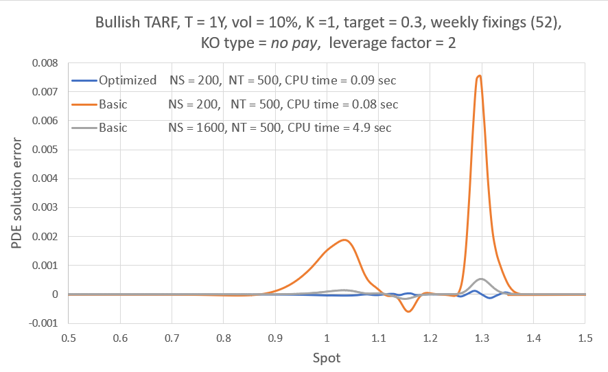
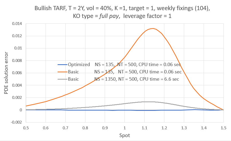
The plots below show the spatial discretization error for the part of the solution that is of interest (the actual solver S-grid extends further) and assuming the accrued amount today is zero, i.e. A = 0. This may mean we are pricing at the time of issue, or at some time during the lifetime of the contract (in which case target stands for "remaining target"). The error profile is obtained by comparing the solution to that from an optimized engine using NS = 6000 and NT = 500 (this has really, really low spatial discretization error, < $10^{-8}$ to be precise). One CPU (Ryzen 5900X) core was used for the timings shown, though if need be the method is easily parallelized. Code is written in C++ and compiled with gcc on Linux. Interest rates are zero.
First we look at a one year contract with weekly fixings/payments and volatility typical of many FX rates. The knockout type is no pay and the leverage factor is two. The optimized version achieves the desired accuracy in 0.09 seconds, while the basic version needs a lot higher spatial resolution and 5 seconds to come close to that.
And now a two year contract and high underlying volatility (more common to precious metals). The knockout type in the case is full pay and the leverage factor is one. In this setting the optimized engine's relative advantage is more pronounced, achieving the desired level of accuracy in 0.06 seconds while the basic engine really struggles here and fails to come close even with a spatial resolution ten times higher. The keen observer will notice the basic problem here immediately.
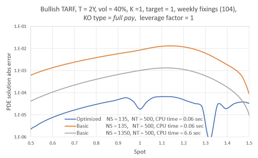
And the same in log scale:
In case it is not clear to all readers, the plots above show that with a single split-second PDE solution we get very low error valuations for the whole range of spot values. This is of course under Black Scholes, but the same level of efficiency should carry over with a volatility model. Thus if the model and/or volatility dynamic assumed allows it, a whole spot ladder calculation should be possible in less than a second.
By the way, if the aim is a single spot valuation, it is often (but not always) preferable to cluster the grid points around the current spot (typical for example when one solves the PDE in log space). In this case one can get higher efficiency still, i.e. same discretization error in even less CPU time.
By the way, if the aim is a single spot valuation, it is often (but not always) preferable to cluster the grid points around the current spot (typical for example when one solves the PDE in log space). In this case one can get higher efficiency still, i.e. same discretization error in even less CPU time.
Some benchmark valuations
While I am at it, why not post some highly accurate benchmark valuations ("benchmark" being a theme in this site). It may be difficult to believe (and in a way pointless, same way as making watches waterproof to depths no human can survive is pointless), but all digits provided should be correct. Perhaps if someone wants to perform basic sanity checks on their TARF pricing engine these can be of some help. So to be clear, assuming fixing and settlement dates coincide and are all dt = 1/52 yrs apart (say forcing an ACT/364 day count with no holidays affecting the weekly fixings dates), flattening the volatility surface and zeroing rates curves, should have you approaching the values below as you increase your pricing engine's resolution (or Monte Carlo iterations).
Table 1. Benchmark valuations for a bullish Target Redemption Forward (TARF) under Black Scholes. In all cases the strike K = 1 and both domestic and foreign rates are zero. The values were obtained with a highly optimized PDE-based pricing engine and all digits shown should be converged, except the last one which may be off by 1 or 2 points.
| Case | T (yrs) | num. fixings | target | lev. factor | KO type | spot | BS vol | TARF value |
| 1 | 1 | 52 | 0.3 | 2 | No Pay | 1.06 | 10% | -0.02096094 |
| 2 | 1 | 52 | 0.5 | 2 | No Pay | 1.06 | 10% | -0.017514630 |
| 3 | 1 | 52 | 0.7 | 2 | No Pay | 1.06 | 10% | 0.035902523 |
| 4 | 1 | 52 | 0.3 | 2 | No Pay | 1.1 | 10% | 0.235120763 |
| 5 | 1 | 52 | 0.3 | 2 | Capped pay | 1.1 | 10% | 0.286424762 |
| 6 | 1 | 52 | 0.3 | 2 | Full pay | 1.1 | 10% | 0.335294058 |
| 7 | 1 | 52 | 0.3 | 1 | No Pay | 1.03 | 10% | -0.29368756 |
| 8 | 1 | 52 | 0.3 | 1 | No pay | 1.1 | 20% | -0.01224772 |
| 9 | 1 | 52 | 0.7 | 1 | No pay | 1.1 | 20% | 0.037345388 |
| 10 | 1 | 52 | 0.7 | 1 | Full pay | 1.1 | 20% | 0.152792822 |
| 11 | 2 | 104 | 0.3 | 1 | No pay | 1.35 | 40% | 0.059232579 |
| 12 | 2 | 104 | 0.5 | 1 | No pay | 1.35 | 40% | 0.315294774 |
| 13 | 2 | 104 | 0.5 | 1 | Full pay | 1.1 | 40% | -3.81704655 |
I will try to follow this up with an update using some volatility model.


 RSS Feed