I decided to run a short numerical experiment the other day after reading, thinking about and trying to offer an intuitive answer to this question: Why does Monte Carlo integration work better than naive numerical integration in high dimensions? The first thing that comes to mind is the "curse of dimensionality": If we want to keep adding points uniformly to a regular grid, then the total number of points increases exponentially with the dimension d and a regular grid is just not a viable option. Say for example that we want to evaluate the integral of a function that depends on the value that some quantity takes on each month of the year. This is a problem of dimension 12. Why? Because each evaluation of the function requires a set of 12 different variables (one for each month). Now if we wanted the same accuracy that we would get in 2-D from say a 10$\times$10 (really coarse!) grid (total grid points $N=100$), we would need a total of $N=10^{12}$, i.e. a trillion points. That would be a lot of work to get a poor result. To get a noticeable increase in accuracy we could go up to 20 points per dimension (which would still be pretty coarse). But even that modest increase would mean that we would then need $N=20^{12}$ points, which is 4096 times more than before! What if our function depended on daily observations (d=365)? Let's not even go there.
The actual question though was not referring to that fundamental problem that regular grids face in high dimensions, but rather asked more specifically: "Why does Monte Carlo's random point selection lead to more accurate integral evaluations than a regular grid approach using the same total number of points N?". This may certainly seem counter-intuitive as one should probably be forgiven to assume that the regular grid point placement should represent the space better than a random one and thus lead to better integral estimation. I looked into this for a second (OK, maybe an hour) and as it happens, maybe surprisingly, the regular grid placement is just not optimal for integration. This was part of my answer:
"Placing points on a regular grid is not the best you can do integration-wise, as it leaves large holes that can be avoided by smarter placement. Think of a 3D regular grid. When you look at it from any side, i.e. when you look at a 2D projection of the points, all the points from the third dimension fall on the same place (they overlap) and thus leave large holes that don't aid the integration. The same happens in higher dimensions, so for better integral estimation any lower-dimensional face (projection) should be as homogeneously and uniformly filled with points as possible, without having points overlapping and creating holes. This is what Quasi-Monte Carlo (QMC) sequences try to do. They place points (deterministically) at locations that (should) avoid leaving them overlapping in lower dimensional projections and for this reason they can beat the regular grid even in 2D and 3D. Think then of Monte Carlo as having the same advantage as QMC (i.e. leaving less glaring holes in lower-dimensional faces, exactly because it lacks that regular structure that is responsible for the holes) but with the extra disadvantage of not placing those points very uniformly and homogeneously (like a regular grid and QMC do). At some point (at around d > 4) the advantage wins over the disadvantage and MC starts beating the regular grid."
So does a typical numerical experiment support the above claims?
Estimating Pi via Monte Carlo evaluation of the volume of an n-ball
Here we are going to do the same, but using a sphere and a 5-D ball instead. The purpose is not really to find $\pi$, but to contrast the efficiency of Monte Carlo integration against a regular Reimann sum and also Quasi Monte Carlo (QMC) as dimension goes up. In other words see which particular point placing strategy gives the better results, i.e. more accurate estimation of $\pi$ for a given number N of sampling points. Monte Carlo places the points in a way that intents to be random (but it's really deterministic since we use computer algorithms (pseudo-random number generators) to generate them. For a Reimann sum we use a regular grid of points that places $N^{1/d}$ points uniformly along each axis. Finally QMC places the points seemingly randomly but really deterministically, seeking some desirable space distribution properties.
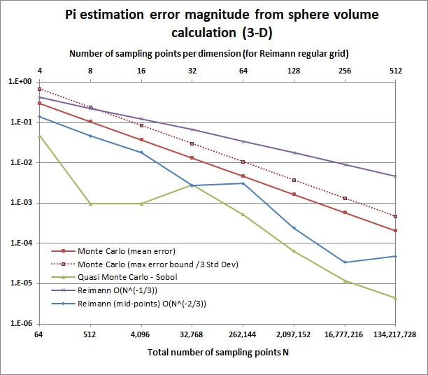
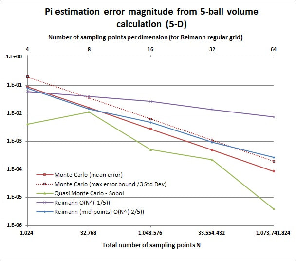
Figures 1 and 2 show the results which seem to be confirming the theory. It can be seen that in 3-D MC (whose error should be of order $O(1/\sqrt{N})$) still loses to the mid-point regular grid ($O(1/{N^{2/3}})$), as expected, and beats the plain regular grid ($O(1/{N^{1/3}})$) again as expected. It can also be seen that QMC beats the mid-point regular grid even in 3-D, as was suggested in my answer above. Presumably because the combination of its uniformity and lower-dimension projection hole-filling properties beats the "perfect" regularity (and point "wasting") of the grid. In 5-D MC (still $O(1/\sqrt{N})$) starts overtaking the mid-point regular grid (now $O(1/{N^{2/5}})$) but still loses to QMC, again as expected.
These graphs might look "wrong" at first sight, the MC error shown as a straight line and the mid-point regular grid a jagged one! That's because I have plotted the mean absolute error for each experiment size N for the MC simulation, instead of plotting just a single simulation's error progression with increasing N. This can be determined numerically for each experiment size, for example obtain 10000 estimations $\hat \pi$ from N=1024-point experiments and find the average of $|\hat \pi-\pi|$. Or we can use this as an opportunity to work a bit of statistics and calculate the expectation $\mathbb E$($|\hat \pi-\pi|$) analytically. Here's how: Calculus tells us that the ratio of the volume of the sphere to the volume of the cube supersribing it is $\pi/6$. So $\pi$ can be estimated as 6 times the proportion of the total N points that will fall into the sphere. One "dart throw" then corresponds to a binomial variate which takes a value of 6 if it (a point) falls into the sphere and zero otherwise. We also know the probability of these outcomes which are $\pi/6$ and $(1-\pi/6)$ respectively. Then the mean of our variate is of course $\pi$ and its variance $\sigma_b^2=$ $(6-\pi)^2(\pi/6)+(0-\pi)^2(1-\pi/6)=$ $2.996657^2$. Then we note that the estimator $\hat\pi$ is just the sum of N such variates divided by N. The Central Limit Theorem tells us that for large N $\hat\pi$ will follow a normal distribution like $\hat\pi\sim \mathcal{N}\left(\mu=\pi,\sigma_{\pi N}^2=\frac{\sigma_b^2}{N}\right)$. It follows that $\hat\pi-\pi\sim \mathcal{N}\left(\mu=0,\sigma_{\pi N}^2=\frac{\sigma_b^2}{N}\right)$. And finally the absolute value of this (i.e. the mean absolute error of our MC experiment using N points) follows a half-normal distribution (special case of the folded normal distribution) and as such will have a mean of $\sigma_{\pi N}\sqrt2/\sqrt\pi$ and variance of $\sigma_{\pi N}^2(1-2/\pi)$. These formulas were used for the MC mean and and indication of the max (3 standard deviations) error in the graph. The mid-point regular grid error on the other hand does show some fluctuation depending on the exact number of points used per dimension. One point more or less leads to a slightly different error magnitude line. The regular grid does not show this.
For the 5-D experiment the equivalent calculus result relates the volume of the 5-ball inscribed in the unit 5-hypercube to $\pi^2$ instead of $\pi$, as $\pi^2/60$. So our dartboard experiment will actually give us an estimate of $\pi^2$. Then the estimate of $\pi$ would just be the square root of that, right? Well almost. Similarly to the sphere case we give a value of 60 if a point falls into the 5-ball and 0 if it doesn't. We also know (a posteriori!) the probability of these outcomes which are $\pi^2/60$ and $(1-\pi^2/60)$ respectively. The single "dart throw" is then a binomial variate with mean $\pi^2$ and variance $\sigma_b^2=(60-\pi^2)^2(\pi^2/60)+$ $(0-\pi^2)^2$ $(1-\pi^2/60)$ $=22.2433624^2$. And when we throw a large number of darts N, then the average of their outcomes follows a normal distribution like $\hat{\pi^2}\sim \mathcal{N}\left(\mu=\pi^2,\sigma_{\pi^2 N}^2=\frac{\sigma_b^2}{N}\right)$. But is $\mathbb E(\sqrt{\hat{\pi^2}})$ equal to $\pi$? Not really. The square root of our $\pi^2$ estimator follows a different distribution with expectation generally smaller than $\pi$, depending on N (Jensen's inequality ensures this is the case, combined with the fact that the square root is a concave function). For N=100, the expectation of our experiment would actually be 3.121. So even if we had say 1 billion estimations of $\pi$ from our 100-dart-throwing into the 5-hypercube experiment, the average of all those estimations would come out as 3.121, not 3.14... So in reality our 5-D experiment does not provide us with an unbiased way of estimating $\pi$, like the 2-D and 3-D experiments do. And assuming we really didn't know the value of $\pi$ then we wouldn't know how big the bias was either. This bias though is rapidly removed as N goes up, for N=1024 the expectation becomes 3.13964 and for N = 1048256 it is 3.141591 (see below how to actually calculate this when we know $\pi$ already). Moreover, this inherent bias in our estimator is always much smaller than the mean absolute error of the experiment (as shown in figures 1 and 2). And as all three methods of point-sampling integration are affected the same, the picture of their comparative performance is not affected.
Finally, out of curiosity, let's see how we can calculate the actual expectation of our 5-D experiment's $\pi$ estimator $\pi_{est}$, $\mathbb E(\pi_{est})$ = $\mathbb E(\sqrt{\hat{\pi^2}})$. Since $\hat{\pi^2}\sim \mathcal{N}\left(\mu=\pi^2,\sigma_{\pi^2 N}^2=\frac{\sigma_b^2}{N}\right)$, the cumulative distribution function (CFD) of $\pi_{est}$ can be seen to be: $F_{\pi_{est}}(x) = $ $\Pr\left(\pi_{est}\leqslant x\right) = \Pr\left(\hat{\pi_2} \leqslant x^2\right) = $ $\Phi\left(\frac{x^2-\pi^2}{\sigma_b/{\sqrt N}}\right) $ where $\Phi$ is the standard normal CDF. The probability density function (PDF) of $\pi_{est}$ is then $ f_{\pi_{est}}(x) = F_{\pi_{est}}^\prime(x)$ $=\frac{2x}{\sigma_b/{\sqrt N}}\phi\left(\frac{x^2-\pi^2}{\sigma_b/{\sqrt N}}\right) $ where $\phi$ is the standard normal PDF. Substituting for $\phi$ we get $ f_{\pi_{est}}(x) = \sqrt {2N/{\pi\sigma_b^2}} \cdot x \cdot exp\left(-N(x^2-\pi^2)^2 / {2\sigma_b^2}\right)$. Then: $$\mathbb E(\pi_{est}) = \int_0^\infty{x \cdot f_{\pi_{est}}(x) dx} = \int_0^\infty{\sqrt {\frac{2N}{\pi\sigma_b^2}} \cdot x^2 \cdot exp\left(\frac{-N(x^2-\pi^2)^2} {2\sigma_b^2}\right)dx}$$ I could not find an analytical solution to this integral, but one can always calculate it numerically with something like Simpson's rule, which is what I did for the figures I quoted above.


 RSS Feed