A few random numerical experiments

Monte Carlo pricing of continuous barrier options with Heston

11/28/2016

Pricing discretely monitored barrier options with Monte Carlo comes natural. One just mimics what would really happen, which is to check if the underlying asset crosses the barrier at specific times only. The "simulation" bias is thus zero. In this case pricing can be accurate if our discretization bias is low (preferably using something better than Euler). But things change when the contract specifies continuous monitoring. The simulation cannot mimic the reality of continuous monitoring since we can only use a finite number of time steps for which we can check if the barrier has been crossed. And one would be forgiven to think that using many time steps (such as corresponding to daily monitoring) would be almost equivalent to true continuous monitoring. But this isn't the case. The probability that the asset could have crossed the barrier in between the implemented time steps is still significant and increasing the number of time steps makes the solution converge only slowly towards the continuous limit. Such a naive simulation will therefore always overestimate the value of a continuous barrier option since it ignores the probability that the option knocks out when we are not looking (i.e. in between time steps).

Now there are generally two ways of reducing, or even getting rid of this simulation bias in special cases. The first is to shift the barrier closer to the asset spot in order to compensate for the times when we "blink". The question is by how much should the barrier be shifted? This was first treated by Broadie, Glasserman & Kou [1], for the Black-Scholes model, where they introduced a continuity correction based on the "magical" number 0.5826. Check it out if you haven't. This trick works pretty well when the spot is not very near the barrier and/or when we have many monitoring dates. But in the opposite case, it can be quite bad and produce errors of 5% or more (Gobet, [2]). This gets worse when there is a steep drop of the value near the barrier, as in a down and out put, or an up and out call with low volatility.

The second way is to use an analytic expression for the probability of hitting the barrier between two realized points in a simulated asset path. This is usually referred to as the probabilistic method, or the Brownian bridge technique, since it uses the probability of Brownian motion hitting a point conditional on two fixed end points. As already implied this probability is known analytically (see [2]) for Brownian motion (and consequently for GBM as well). So for the usual GBM asset model (Black-Scholes), this technique can remove the simulation bias completely. One can just use the probability directly, multiplying each path's payoff with the total path survival probability (based on the survival probability of each path segment S[i], S[i+1]). This is preferable when applicable since it results in lower simulation variance. Alternatively one can sample this probability through a uniform variate draw and use it to decide whether the barrier has been crossed or not. This is the only option when we have to perform regression for American exercise. All this is implemented for the Black-Scholes model in the current version of the pricer which you can download here and check this technique in action (see also here). Below is just a simple example.

As can be seen the probabilistic method (enabled by checking "continuous monitoring") enables exact Monte Carlo pricing of this continuously monitored up and out call (for which of course the exact analytic solution is available and is shown as well and marked by the blue line). By contrast, the barrier-shifting method misprices this option by quite some margin (3.4%), as can be seen in the second slide where the probabilistic correction is unchecked and instead the barrier has been shifted downwards according to BGK's (not so magic here) formula.

Same trick but now with Heston

Now the analytical (Brownian Bridge) hitting probability is only available for a BM/GMB process. But what if we have a not so simple process? Well, as long as the discretization scheme we use for the asset makes it locally BM/GBM (always the case when we use Euler to discretize S, or log(S)), then we can still use this trick. It won't remove the simulation bias completely, but it may do a good job nonetheless. So I thought I'd try it with Heston and see how it performs. I only have two discretization schemes set up, the Full Truncation Euler and the Quadratic Exponential (with Martingale correction). Both are considered short-stepping schemes, though QE-M can do pretty well with long steps as well, especially for vanillas, not so much for path-dependent options. FTE definitely needs short time steps to give acceptable accuracy. Both schemes though use normal increments to march log(S) in time, conditional on the variance process path realization which comes first. So we can still use our BB probability formulas like we did with the Black-Scholes model. The only catch here is that the BB formulas assume constant variance and we have stochastic variance instead (not to mention correlation between the variance and the asset processes). That's why it will only be an approximation. For each asset path segment S[i], S[i+1] we have the corresponding variances v[i] and v[i+1] which we can use in the BB probability formula. Now since we want to see to what extent the simulation (monitoring) bias can be removed, we'd like to get the discretization bias out of the way so that it doesn't cloud the results. For this reason I used the QE-M scheme with daily time steps. The test cases considered are in table 1, all Up and Out calls for 5 different Heston parameter sets, chosen from the literature without too much thought, although I did try to set up case 4 to be a kind of torture test and the Feller condition is violated in case 7. Those two cases are the ones with the largest error as can be seen in table 2. The "exact" price for the continuously monitored options was calculated by the PDE/FDM solver presented in the previous post. The price when the monitoring is discrete (daily) is also shown for comparison. A large number of Sobol-driven paths were used so that the (Q)MC prices shown are converged to all digits shown (last digit may be off by one). As can be seen, it seems that the method yields accurate approximations of the correct continuous price indeed, the highest error being 0.35%. Note also that even with daily monitoring the discrete version prices (plain MC, no correction) are quite different from the continuous ones (up to 37%), showcasing the need for the probabilistic (BB) correction when it's a continuous barrier price we're after.

Table 1. Test cases parameter sets for Up and Out call options.

	κ	η	σ	ρ	rd	rf	T	K	U	So	vo
Case 1	5	0.16	0.9	0.1	0.1	0	0.25	100	120	100	0.0625
Case 2	5	0.16	0.9	0.1	0.1	0	0.25	100	135	130	0.0625
Case 3	1.5	0.04	0.3	-0.9	0.025	0	0.25	100	115	100	0.0625
Case 4	1.5	0.04	0.3	-0.9	0.025	0	0.25	100	135	130	0.0625
Case 5	3	0.12	0.04	0.6	0.01	0.04	0.25	100	120	100	0.09
Case 6	2.5	0.06	0.5	-0.1	0.0507	0.0469	0.5	100	120	100	0.0625
Case 7	6.21	0.019	0.61	-0.7	0.0319	0	0.5	100	110	100	0.010201

Table 2. Effectiveness of Monte Carlo with the Probabilistic Continuity Correction for the pricing of cont. monitored barrier options under the Heston model. The MC prices are converged and the time-discretization error is negligible.

	Solver	Price	Difference
Case 1	PDE/FDM cont. monitoring (exact)	1.8651	-
	MC with 63 timesteps & PCC	1.8652	0.01%
	Plain MC with 63 timesteps	2.1670	16%
Case 2	PDE/FDM cont. monitoring (exact)	2.5021	-
	MC with 63 timesteps & PCC	2.5032	0.04%
	Plain MC with 63 timesteps	3.4159	37%
Case 3	PDE/FDM cont. monitoring (exact)	2.1312	-
	MC with 63 timesteps & PCC	2.1277	-0.16%
	Plain MC with 63 timesteps	2.3369	10%
Case 4	PDE/FDM cont. monitoring (exact)	3.6519	-
	MC with 63 timesteps & PCC	3.6394	-0.34%
	Plain MC with 63 timesteps	4.6731	28%
Case 5	PDE/FDM cont. monitoring (exact)	1.6247	-
	MC with 63 timesteps & PCC	1.6249	0.01%
	Plain MC with 63 timesteps	1.8890	16%
Case 6	PDE/FDM cont. monitoring (exact)	1.7444	-
	MC with 125 timesteps & PCC	1.7438	-0.03%
	Plain MC with 125 timesteps	1.9209	10.1%
Case 7	PDE/FDM cont. monitoring (exact)	1.9856	-
	MC with 125 timesteps & PCC	1.9790	-0.33%
	Plain MC with 125 timesteps	2.0839	4.95%

Finally regarding the variance value used in the probability formulas, my brief testing showed that the best results were obtained when using the variance corresponding to the one of the two nodes S[i] and S[i+1] which is closer to the barrier. This was the choice for the results of Table 2.
Once I set up a more accurate long stepping discretization scheme, I may test to see how well this approximation holds when one uses fewer/longer time steps.

References

[1] Broadie M, Glasserman P, & Kou S. A continuity correction for discrete barrier options, Mathematical Finance, Vol. 7 (4) (1997), pp. 325-348.
[2] Emmanuel Gobet. Advanced Monte Carlo methods for barrier and related exotic options. Bensoussan A., Zhang Q. et Ciarlet P. Mathematical Modeling and Numerical Methods in Finance, Elsevier, pp.497-528, 2009, Handbook of Numerical Analysis

0 Comments

Old-fashioned Heston pricer vs the state of the art

8/9/2016

1 Comment

My old option pricer (which you can download "refurbished" here) had a basic stochastic volatility (Heston) solver which never really passed the testing phase, so I kept it hidden. Besides, it was using SOR to solve the full system at each time-step, so it can't compete with the modern "state of the art" ADI variants. Or can it?

Well I decided to give it another try and see how it compares really after a few optimizing tweaks.

The Heston Partial Differential Equation

We are trying to solve the following PDE by discretizing it with the finite difference method:

$$\frac{\partial V}{\partial t} = \frac{1}{2} S^2 \nu\frac{\partial^2 V}{\partial S^2}+\rho \sigma S \nu \frac{\partial^2 V}{\partial S \partial \nu} + \frac{1}{2}\sigma^2\nu\frac{\partial^2 V}{\partial \nu^2} + (r_d-r_f)S \frac{\partial V}{\partial S}+ \kappa (\eta-\nu) \frac{\partial V}{\partial \nu}-r_d V $$
where $\nu$ is the variance of the underlying asset $S$ returns, $\sigma$ is the volatility of the $\nu$ process, $\rho$ the correlation between the $S$ and $ \nu$ processes and $\eta$ is the long-term variance to which $\nu$ is mean-reverting with rate $\kappa$. Here $S$ follows geometrical Brownian motion and $\nu$ the CIR (Cox, Ingersoll and Ross) mean-reverting process.

Time-discretization: Four-level fully implicit (4LFI, or FI-BDF3)

After we discretize the PDE we are left with an algebraic system of equations relating the values at each grid point (i,j) with those at its neighboring points. With the standard implicit scheme (Euler) the values at time n+1 are found as $ V_{i,j}^{(n+1)} = (B \cdot dt+V_{i,j}^{(n)})/(1-a_{i,j} \cdot dt) $ for each grid point (i,j). $B$ is a linear combination of $ V^{(n+1)} $ at (i,j)'s neighboring points and $a_{i,j}$ the coefficient of $ V_{i,j} $ arising from the spatial discretization. So we need to solve the system of unknowns $ V_{i,j}^{(n+1)} $.
The 3LFI (otherwise known as implicit BDF2) scheme just adds a little information from time point n-1 and can simply be described as: $ V_{i,j}^{(n+1)} = (B \cdot dt+2 \cdot V_{i,j}^{(n)}-0.5 \cdot V_{i,j}^{(n-1)})/(1.5-a_{i,j} \cdot dt) $, $a_{i,j}$ and $B$ being the same as before. This little addition makes the 3LFI/BDF2 scheme second order in time, whereas the standard implicit is only first order.

This scheme is strongly A-stable (?), so unlike something like Crank-Nicolson (CN) it has built-in oscillation-damping on top of being unconditionally stable. So I tested this first and while it worked pretty well, I found that it produced slightly larger errors than CN. That is while they're both second-order accurate, CN's error-constant was lower. Which is not surprising, central discretizations often produce higher accuracy than their one-sided counterparts of the same order. Moreover it was notably less time-converged compared to the ADI schemes using the same number of time-steps.

So I decided to go for higher-spec. Especially since it comes really cheap in terms of implementation. Adding an extra time-point gives us the 4LFI or BDF3 scheme, which is third order:
$$ BDF3 : \quad V_{i,j}^{(n+1)} = \left (B \cdot dt+3 \cdot V_{i,j}^{(n)}-\frac 3 2 \cdot V_{i,j}^{(n-1)}+\frac 1 3 \cdot V_{i,j}^{(n-2)}\right)/\left(\frac {11} 6 - a_{i,j} \cdot dt\right) \qquad (1)$$
While such a scheme is no longer strictly unconditionally stable (it's almost A-stable), it should still be almost as good as and should preserve the damping qualities of 3LFI/BDF2. As it happens, the results it produces are significantly more accurate than both the 3LFI/BDF2 and the ADI schemes for any number of time-steps. Third order beats second order easily here, despite being a one-sided one. Finally as an added bonus, it adds a little to the diagonal dominance of the iteration matrix of the SOR solver so it helps convergence as well.

Now since this is a multi-step scheme (it needs the values not just from the previous time level but also from two levels before that), we need to use something different for the first couple of time steps, a starting procedure. For the very first step we need a two-level (single step) scheme. We cannot use CN because this will allow spurious oscillations to occur given the non-smooth initial conditions of option payoff functions. Instead one can use the standard Implicit Euler scheme plus local extrapolation: we first use the IE scheme for 4 sub-steps of size dt/4 to get the values $ V_{fine}^1$ at the end of the first time step. We then repeat, this time using 2 sub-steps of size dt/2 to obtain $ V_{coarse}^1$ and get the final composite values for the first time step as $(4V_{fine}^1-V_{coarse}^1)/3 $. For the second time step we just use the 3LFI/BDF2.

Space-discretization and boundary conditions

Central finite differences are used for everything, except again for the v = 0 boundary, where we need to use a one-sided (three-point) upwind second-order discretization for the first v-derivative. Hout & Foulon [1] also use that upwind discretization in some cases where v > 1, but I stick to the central formula here. And of course I make sure that the strike falls in the middle between two grid points, which is something that occasionally people seem to neglect in a few publications I've seen. Suitable Neumann and/or Dirichlet boundary conditions are used everywhere except for the v = 0 variance boundary where we require that the PDE itself (with many terms being zero there) is satisfied, all as described in Hout & Foulon [1].

System solver

I used successive over-relaxation (SOR) to solve the resulting system because it's so easy to set up and accommodate early exercise features. On the other hand it is in general quite slow and moreover its speed may depend significantly on the chosen relaxation factor $\omega$. This is where the hand-made part comes in. I am using an SOR variant called TSOR together with a simple algorithm that adjusts $\omega$ as it goes, monitoring proceedings for signs of divergence as well (e.g. residual increasing instead of decreasing). I am not 100% sure my implementation is bug free, but it seems that the resulting SOR iteration matrix is not always such that it leads to convergence. There's a maximum $\omega$ which presumably makes the spectral radius of the iteration matrix less than one, but I've not pursued any further analysis on that, relying instead on the heuristic algorithm to keep it safe and close to optimal. All in all the modifications compared to the standard SOR amount to a few lines of code. I may write details of TSOR in another post but for the moment let's just say that it speeds things up about 3 times compared to standard SOR, plus it seems less dependent on $\omega$.

1 Comment

Higher-order accuracy: Richardson extrapolation vs native higher-order scheme in 2D

4/15/2016

1 Comment

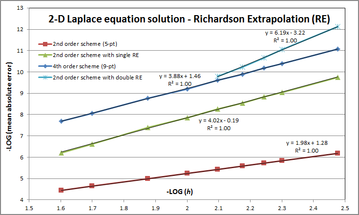
The other day I noticed this interesting graph lying in a corner on my desktop and I thought I might as well post it here. It was part of the background tests I did while I was calculating the benchmark results for the driven cavity flow problem. In order to have first an idea of how well I could expect my 2D Richardson extrapolation (RE) set-up to work under "perfect" conditions, I thought I would apply it first on a simpler, more benign problem. To this end I solved the 2D Laplace equation for the steady state temperature distribution on a unit square plate, with the top side maintained at a constant unit temperature and the remaining three sides at zero (Dirichlet-type boundary conditions). This problem has an analytic solution in the form of an infinite (Fourier) series, which we can use to calculate the error of different numerical methods/schemes. So I was curious to see to what extent can RE improve on a second-order scheme's accuracy and especially how the results fare against a proper, natively fourth-order scheme.
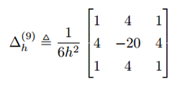
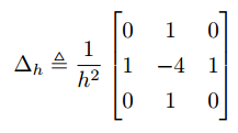
I remember reading long time ago that RE will indeed improve the accuracy of a second-order scheme, increase its convergence order to $O({h^4})$ if implemented properly, but will not produce as accurate results as a scheme that is fourth-order accurate ($O({h^4})$ truncation error) by design. I had seen examples of this in 1D, but I hadn't seen results for 2D so I thought I'd do this test. Let's imagine for now that grid points are uniformly spaced, as was indeed the case in this test. The second-order scheme used is the standard 5-point stencil and the fourth-order scheme is the fantastic 9-point compact stencil.

$O({h^2})$ scheme, 5-point stencil

$O({h^4})$ scheme, 9-point stencil

RE implementation

The RE solution is a linear combination of two solutions calculated on two different grids (representing the solution on two different sets of discrete points, or nodes if you prefer). In order to combine the two solutions we need to have them at the same locations, so if there's no common set of points we then need to somehow bring/project one solution onto the grid of the other. So we need to interpolate. Usually people will perform RE by combining the solution on a grid with say N steps in each dimension (h=1/N), with that on a grid with half or double the spacing h. This way there's no need to use interpolation if we're projecting our final RE result on the coarser grid, because the finer grid already has the solution on all the coarser grid's points. If we want the RE results "printed" on the finer grid's resolution instead, then we need to interpolate in order to "guess" what the coarser grid's solution is at those extra points that the finer grid has. In the 2D case this means we would need to produce N$\times$N values based on information from only 25% as many (the 0.5$\times$0.5$\times$N$\times$N values of our coarse grid).

I prefer keeping the two grid resolutions closer to each other. Too close is not good either though because then the two solutions are not "distinct" enough and the extrapolation loses accuracy. My tests here showed that a spacing ratio of 0.85 is about right. In this case when we interpolate the results of the coarser (0.85$\times$0.85$\times$N$\times$N) grid "upwards", we generate our N$\times$N values now using 72% as many values, as opposed to 25% in the half spacing case. We now definitely need to interpolate of course because the two grids' sets of points are going to be distinct. Simple (2D) local polynomial interpolation was used here. The important detail is that the interpolating polynomial accuracy (degree) needs to be the same or higher than that which we expect to obtain from the extrapolation. I used sixth-degree polynomials for the results in the graph below. That worked fine because the combination of the smoothly-varying field and the high grid resolutions meant that any 7 contiguous points used to fit the polynomials were always pretty much on a straight line. When the function we are trying to find a solution for is less benign, using such high-order polynomials will in general make things worse due to Runge's phenomenon. We would then need to cramp many more grid points in order to avoid this problem. In practice, non-uniform grids are often used anyway in order to properly resolve areas of steep gradients by concentrating more points there, regardless of whether we plan to extrapolate or not.

Results

So here's the graph I was talking about. It shows how the average absolute error (across all solution grid points) falls as we make the grid spacing h smaller. Well not exactly all grid points. I've actually excluded the first 5% from the top side of the square domain downwards. The reason is that due to the singularities in the top two corners (the boundary conditions there change discontinuously from unit at the top to zero at the sides), the solution in their vicinity misbehaves. Here we don't care about that so in order to get a clean picture of the orders of convergence under "normal" circumstances, I left those points out of the average error calculation. So on to the results. Expectations were generally confirmed, or even exceeded in the case of the double RE. The latter basically combines two (fourth-order) RE results to extrapolate to a theoretically sixth-order accurate result. With double RE being an extrapolation based on other (single RE) extrapolations (all of which based on interpolations!), I was not sure at all I'd get anywhere near sixth-order. But sure enough, $O({h^{6+}})$ was obtained for this smooth field. As expected, even though the single RE actually achieved slightly better order of convergence than the native fourth-order 9-point scheme in this case, the actual error it produced was significantly higher, about 22 times higher to be exact for the range of h used. The double RE though managed to beat the fourth-order scheme for actual accuracy achieved, producing lower errors when the grid is reasonably fine (for h < 0.01 roughly).

1 Comment

Monte Carlo wins: How can randomly placed points perform better than a regular grid for integral evaluation in higher dimensions?

10/8/2015

2 Comments

I decided to run a short numerical experiment the other day after reading, thinking about and trying to offer an intuitive answer to this question: Why does Monte Carlo integration work better than naive numerical integration in high dimensions? The first thing that comes to mind is the "curse of dimensionality": If we want to keep adding points uniformly to a regular grid, then the total number of points increases exponentially with the dimension d and a regular grid is just not a viable option. Say for example that we want to evaluate the integral of a function that depends on the value that some quantity takes on each month of the year. This is a problem of dimension 12. Why? Because each evaluation of the function requires a set of 12 different variables (one for each month). Now if we wanted the same accuracy that we would get in 2-D from say a 10$\times$10 (really coarse!) grid (total grid points $N=100$), we would need a total of $N=10^{12}$, i.e. a trillion points. That would be a lot of work to get a poor result. To get a noticeable increase in accuracy we could go up to 20 points per dimension (which would still be pretty coarse). But even that modest increase would mean that we would then need $N=20^{12}$ points, which is 4096 times more than before! What if our function depended on daily observations (d=365)? Let's not even go there.

The actual question though was not referring to that fundamental problem that regular grids face in high dimensions, but rather asked more specifically: "Why does Monte Carlo's random point selection lead to more accurate integral evaluations than a regular grid approach using the same total number of points N?". This may certainly seem counter-intuitive as one should probably be forgiven to assume that the regular grid point placement should represent the space better than a random one and thus lead to better integral estimation. I looked into this for a second (OK, maybe an hour) and as it happens, maybe surprisingly, the regular grid placement is just not optimal for integration. This was part of my answer:

"Placing points on a regular grid is not the best you can do integration-wise, as it leaves large holes that can be avoided by smarter placement. Think of a

3D

regular grid. When you look at it from any side, i.e. when you look at a

2D

projection of the points, all the points from the third dimension fall on the same place (they overlap) and thus leave large holes that don't aid the integration. The same happens in higher dimensions, so for better integral estimation any lower-dimensional face (projection) should be as homogeneously and uniformly filled with points as possible, without having points overlapping and creating holes. This is what Quasi-Monte Carlo (QMC) sequences try to do. They place points (deterministically) at locations that (should) avoid leaving them overlapping in lower dimensional projections and for this reason they can beat the regular grid even in

2D

and 3

3D

. Think then of Monte Carlo as having the same advantage as QMC (i.e. leaving less glaring holes in lower-dimensional faces, exactly because it lacks that regular structure that is responsible for the holes) but with the extra disadvantage of not placing those points very uniformly and homogeneously (like a regular grid and QMC do). At some point (at around

d>4

) the advantage wins over the disadvantage and MC starts beating the regular grid."

So does a typical numerical experiment support the above claims?

Estimating Pi via Monte Carlo evaluation of the volume of an n-ball

Let's take a closer look at the introductory Monte Carlo experiment of trying to calculate the value of $\pi$ through a "dartboard" approach. This is usually done by estimating the ratio of the area of a circle to the area of the square that just superscribes it, by randomly "throwing darts" (simulated by generating random point coordinates (x,y)) inside the square and calculating the proportion of the total points that fall into the inscribed circle. This ratio can also be calculated through calculus in terms of $\pi$ as $\pi/4$. At this point the "unknown" $\pi$ is defined as the ratio of a circle's circumference to its diameter.

Here we are going to do the same, but using a sphere and a 5-D ball instead. The purpose is not really to find $\pi$, but to contrast the efficiency of Monte Carlo integration against a regular Reimann sum and also Quasi Monte Carlo (QMC) as dimension goes up. In other words see which particular point placing strategy gives the better results, i.e. more accurate estimation of $\pi$ for a given number N of sampling points. Monte Carlo places the points in a way that intents to be random (but it's really deterministic since we use computer algorithms (pseudo-random number generators) to generate them. For a Reimann sum we use a regular grid of points that places $N^{1/d}$ points uniformly along each axis. Finally QMC places the points seemingly randomly but really deterministically, seeking some desirable space distribution properties.

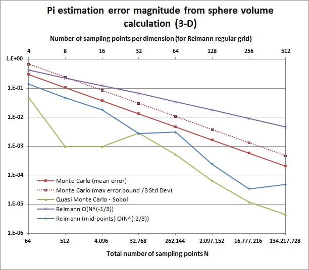
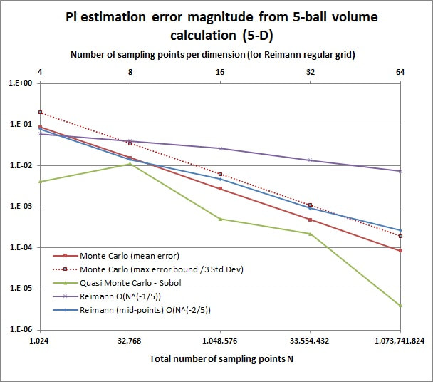
Figures 1 and 2 show the results which seem to be confirming the theory. It can be seen that in 3-D MC (whose error should be of order $O(1/\sqrt{N})$) still loses to the mid-point regular grid ($O(1/{N^{2/3}})$), as expected, and beats the plain regular grid ($O(1/{N^{1/3}})$) again as expected. It can also be seen that QMC beats the mid-point regular grid even in 3-D, as was suggested in my answer above. Presumably because the combination of its uniformity and lower-dimension projection hole-filling properties beats the "perfect" regularity (and point "wasting") of the grid. In 5-D MC (still $O(1/\sqrt{N})$) starts overtaking the mid-point regular grid (now $O(1/{N^{2/5}})$) but still loses to QMC, again as expected.

Figure 1. Pi estimation absolute error through calculation of a sphere volume with different sampling point placement strategies.

Figure 2. Pi estimation absolute error through calculation of a 5-ball volume with different sampling point placement strategies.

These graphs might look "wrong" at first sight, the MC error shown as a straight line and the mid-point regular grid a jagged one! That's because I have plotted the mean absolute error for each experiment size N for the MC simulation, instead of plotting just a single simulation's error progression with increasing N. This can be determined numerically for each experiment size, for example obtain 10000 estimations $\hat \pi$ from N=1024-point experiments and find the average of $|\hat \pi-\pi|$. Or we can use this as an opportunity to work a bit of statistics and calculate the expectation $\mathbb E$($|\hat \pi-\pi|$) analytically. Here's how: Calculus tells us that the ratio of the volume of the sphere to the volume of the cube supersribing it is $\pi/6$. So $\pi$ can be estimated as 6 times the proportion of the total N points that will fall into the sphere. One "dart throw" then corresponds to a binomial variate which takes a value of 6 if it (a point) falls into the sphere and zero otherwise. We also know the probability of these outcomes which are $\pi/6$ and $(1-\pi/6)$ respectively. Then the mean of our variate is of course $\pi$ and its variance $\sigma_b^2=$ $(6-\pi)^2(\pi/6)+(0-\pi)^2(1-\pi/6)=$ $2.996657^2$. Then we note that the estimator $\hat\pi$ is just the sum of N such variates divided by N. The Central Limit Theorem tells us that for large N $\hat\pi$ will follow a normal distribution like $\hat\pi\sim \mathcal{N}\left(\mu=\pi,\sigma_{\pi N}^2=\frac{\sigma_b^2}{N}\right)$. It follows that $\hat\pi-\pi\sim \mathcal{N}\left(\mu=0,\sigma_{\pi N}^2=\frac{\sigma_b^2}{N}\right)$. And finally the absolute value of this (i.e. the mean absolute error of our MC experiment using N points) follows a half-normal distribution (special case of the folded normal distribution) and as such will have a mean of $\sigma_{\pi N}\sqrt2/\sqrt\pi$ and variance of $\sigma_{\pi N}^2(1-2/\pi)$. These formulas were used for the MC mean and and indication of the max (3 standard deviations) error in the graph. The mid-point regular grid error on the other hand does show some fluctuation depending on the exact number of points used per dimension. One point more or less leads to a slightly different error magnitude line. The regular grid does not show this.

For the 5-D experiment the equivalent calculus result relates the volume of the 5-ball inscribed in the unit 5-hypercube to $\pi^2$ instead of $\pi$, as $\pi^2/60$. So our dartboard experiment will actually give us an estimate of $\pi^2$. Then the estimate of $\pi$ would just be the square root of that, right? Well almost. Similarly to the sphere case we give a value of 60 if a point falls into the 5-ball and 0 if it doesn't. We also know (a posteriori!) the probability of these outcomes which are $\pi^2/60$ and $(1-\pi^2/60)$ respectively. The single "dart throw" is then a binomial variate with mean $\pi^2$ and variance $\sigma_b^2=(60-\pi^2)^2(\pi^2/60)+$ $(0-\pi^2)^2$ $(1-\pi^2/60)$ $=22.2433624^2$. And when we throw a large number of darts N, then the average of their outcomes follows a normal distribution like $\hat{\pi^2}\sim \mathcal{N}\left(\mu=\pi^2,\sigma_{\pi^2 N}^2=\frac{\sigma_b^2}{N}\right)$. But is $\mathbb E(\sqrt{\hat{\pi^2}})$ equal to $\pi$? Not really. The square root of our $\pi^2$ estimator follows a different distribution with expectation generally smaller than $\pi$, depending on N (Jensen's inequality ensures this is the case, combined with the fact that the square root is a concave function). For N=100, the expectation of our experiment would actually be 3.121. So even if we had say 1 billion estimations of $\pi$ from our 100-dart-throwing into the 5-hypercube experiment, the average of all those estimations would come out as 3.121, not 3.14... So in reality our 5-D experiment does not provide us with an unbiased way of estimating $\pi$, like the 2-D and 3-D experiments do. And assuming we really didn't know the value of $\pi$ then we wouldn't know how big the bias was either. This bias though is rapidly removed as N goes up, for N=1024 the expectation becomes 3.13964 and for N = 1048256 it is 3.141591 (see below how to actually calculate this when we know $\pi$ already). Moreover, this inherent bias in our estimator is always much smaller than the mean absolute error of the experiment (as shown in figures 1 and 2). And as all three methods of point-sampling integration are affected the same, the picture of their comparative performance is not affected.

Finally, out of curiosity, let's see how we can calculate the actual expectation of our 5-D experiment's $\pi$ estimator $\pi_{est}$, $\mathbb E(\pi_{est})$ = $\mathbb E(\sqrt{\hat{\pi^2}})$. Since $\hat{\pi^2}\sim \mathcal{N}\left(\mu=\pi^2,\sigma_{\pi^2 N}^2=\frac{\sigma_b^2}{N}\right)$, the cumulative distribution function (CFD) of $\pi_{est}$ can be seen to be: $F_{\pi_{est}}(x) = $ $\Pr\left(\pi_{est}\leqslant x\right) = \Pr\left(\hat{\pi_2} \leqslant x^2\right) = $ $\Phi\left(\frac{x^2-\pi^2}{\sigma_b/{\sqrt N}}\right) $ where $\Phi$ is the standard normal CDF. The probability density function (PDF) of $\pi_{est}$ is then $ f_{\pi_{est}}(x) = F_{\pi_{est}}^\prime(x)$ $=\frac{2x}{\sigma_b/{\sqrt N}}\phi\left(\frac{x^2-\pi^2}{\sigma_b/{\sqrt N}}\right) $ where $\phi$ is the standard normal PDF. Substituting for $\phi$ we get $ f_{\pi_{est}}(x) = \sqrt {2N/{\pi\sigma_b^2}} \cdot x \cdot exp\left(-N(x^2-\pi^2)^2 / {2\sigma_b^2}\right)$. Then: $$\mathbb E(\pi_{est}) = \int_0^\infty{x \cdot f_{\pi_{est}}(x) dx} = \int_0^\infty{\sqrt {\frac{2N}{\pi\sigma_b^2}} \cdot x^2 \cdot exp\left(\frac{-N(x^2-\pi^2)^2} {2\sigma_b^2}\right)dx}$$ I could not find an analytical solution to this integral, but one can always calculate it numerically with something like Simpson's rule, which is what I did for the figures I quoted above.

2 Comments

Forward>>

Monte Carlo pricing of continuous barrier options with Heston

References

Old-fashioned Heston pricer vs the state of the art

Higher-order accuracy: Richardson extrapolation vs native higher-order scheme in 2D

Monte Carlo wins: How can randomly placed points perform better than a regular grid for integral evaluation in higher dimensions?

Estimating Pi via Monte Carlo evaluation of the volume of an n-ball

Author

Archives

Categories

Monte Carlo pricing of continuous barrier options with Heston

References

Old-fashioned Heston pricer vs the state of the art

Higher-order accuracy: Richardson extrapolation vs native higher-order scheme in 2D

Monte Carlo wins: How can randomly placed points perform better than a regular grid for integral evaluation in higher dimensions?﻿

Estimating Pi via Monte Carlo evaluation of the volume of an n-ball

Author

Archives

Categories

Monte Carlo wins: How can randomly placed points perform better than a regular grid for integral evaluation in higher dimensions?